STK Premium (Space) or STK Enterprise
You can obtain the necessary licenses for this tutorial by contacting AGI Support at support@agi.com or 1-800-924-7244.
Version 13.0 of the Ansys Systems Tool Kit® (STK®) digital mission engineering software and Ansys Orbit Determination Tool Kit (ODTK®) orbital measurement processing software are required to complete this tutorial.
The results of the tutorial may vary depending on the user settings and data enabled (online operations, terrain server, dynamic Earth data, etc.). It is acceptable to have different results.
Capabilities covered
This lesson covers the following capabilities of the Ansys Systems Tool Kit® (STK®) digital mission engineering software:
- STK Pro
- Astrogator
Problem statement
Engineers and operators need to analyze the results of a launch into low earth Orbit (LEO) that did not go exactly as planned. You have the nominal trajectory, which you planned using the STK/Astrogator® capability, but you need to understand the current state of the satellite from available tracking data so you can recompute the maneuvers needed for a successful Hohmann transfer into your targeted geostationary orbit (GEO).
Solution
Use the Ansys Orbit Determination Tool Kit (ODTK®) orbital measurement processing software to process the tracking measurements and create a post-launch flight dynamics record, which you can pass to the STK software for further analysis. Use the flight dynamics record to recompute the maneuvers for the satellite's actual trajectory. Create acceleration history (*.accelhist) files to feed back into the ODTK application to analyze the results of the planned maneuvers. The purpose of this exercise is to teach you how to make the STK software's Astrogator capability and the ODTK software work together, not how to build Astrogator or ODTK scenarios.
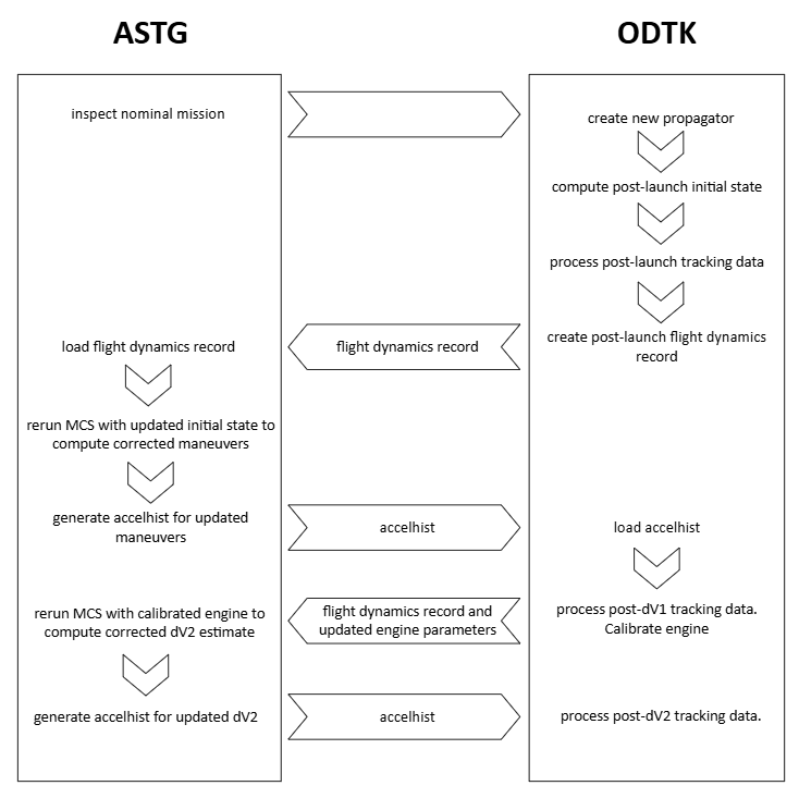
STK-ODTK workflow diagram
What you will learn
Upon completion of this tutorial, you will be able to:
- Use the ODTK application's component browser
- Create flight dynamics records in the ODTK application
- Share propagators and flight dynamics records between the STK and ODTK applications
- Create and use acceleration history files
Video guidance
Watch the following video. Then follow the steps below, which incorporate the systems and missions you work on (sample inputs provided).
Opening the starter STK scenario
A partially created scenario containing the nominal launch trajectory designed using the Astrogator capability has been built for you and is included with the STK software installation.
- Launch the STK application (
 ).
). - Click Open a Scenario (
 ) in the Welcome to STK dialog box.
 - Browse to <Install Dir>\Data\Resources\stktraining\VDFs.
- Select STK_ODTK.vdf.
- Click .
Saving the VDF as an STK scenario
Save and extract the VDF data in the form of a scenario folder. When you save a VDF in the STK application, it will save in its originating format. That is, if you open a VDF, the default save format will be a VDF (*.vdf). If you want to save and extract a VDF as a scenario folder, you must change the file format by using the Save As feature. This will create a permanent scenario file complete with child objects and any additional files packaged with the VDF.
- Select the File menu.
- Select Save As....
- Select the STK User folder in the navigation panel when the Save As dialog box opens.
- Select the STK_ODTK folder.
- Click .
- Select Scenario Files (*.sc) as the Save as type.
- Select the STK_ODTK Scenario file in the file browser.
- Click .
- Click when the Confirm Save As dialog box opens to overwrite the existing scenario file in the folder and to save your scenario.
A scenario folder with the same name as the VDF was created for you when you opened the VDF in the STK application. This folder contains the temporarily unpacked files from the VDF.
When saving a VDF as a scenario folder, you should extract its contents to the scenario folder the STK application automatically creates for you in the STK User folder. See the
Save (![]() ) your scenario often!
) your scenario often!
Nominal trajectory
Reviewing the starter STK scenario
Review the starter scenario to get a better understanding of the nominal launch trajectory.
- Right-click on NominalMission (
 ) in the Object Browser.
 - Select Properties (
 ) in the shortcut menu.
 - Ensure the Basic - Orbit page is selected.
- Review the Mission Control Sequence (MCS).
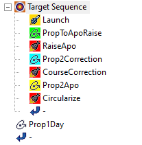
- A Launch (
 ) segment, Launch, into LEO
 - A Propagate (
 ) segment, PropToApoRaise, to the apogee-raising maneuver
 - A Maneuver (
 ) segment, RaiseApo, to raise the apogee
 - A Course-correction Maneuver () segment, CourseCorrection, which is set to 0 for now, but may become necessary later
- Another Propagate () segment, Prop2Apo, which propagates the orbit to circularization
- A final Maneuver () segment, Circularize, which will bring the satellite into a circular, non-inclined orbit 10 km below GEO altitude so the satellite can drift to the desired longitude
- Click to close the Properties Browser without saving any changes.
- Keep the STK application open.
The Astrogator satellite consists of several segments nested in a Target Sequence:
The other two satellites in the scenario are similar and will be used later on in the tutorial. Instead of starting from launch, they start with initial states from later in the mission, the properties of which you will calculate using the ODTK software.
NominalMission MCS
Opening the starter ODTK scenario
Open and review the starter ODTK scenario.
- Launch the ODTK application (
 ).
). - Select the File menu.
- Select Open... ().
- Browse to <Install Dir>\Data\Resources\odtktraining\scenarios.
- Select ODTK_STK.sco.
- Click .
- Review the scenario.
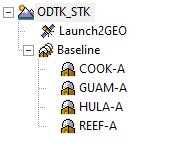
You are using the Baseline ![]() ) object, which provides a convenient way of grouping one or more facilities. Four
) object, which provides a convenient way of grouping one or more facilities. Four ![]() ) objects in the Tracking System model remote tracking stations in the Satellite Control Network, which provide range, Doppler, azimuth and elevation measurements. A post-launch
) objects in the Tracking System model remote tracking stations in the Satellite Control Network, which provide range, Doppler, azimuth and elevation measurements. A post-launch ![]() ), has already been created for you.
), has already been created for you.
ODTK Scenario Setup
Saving the ODTK scenario
Save a copy of the ODTK starter scenario to a subfolder in your STK Scenario folder.
- Select Save As... in the File menu.
- Navigate to your User folder (e.g., C:\Users\<username>\Documents\STK_ODTK 13.
- Open the STK_ODTK Scenario folder.
- Right-click in the file and folder listing.
- Select New in the shortcut menu.
- Select Folder in the New submenu.
- Rename the new folder ODTK_STK.
- Select the Enter key.
- Click .
- Click .
Saving the ODTK scenario to a separate subfolder prevents any files like propagators and flight dynamics record from being accidentally overwritten as you build your scenarios.
Updating the ODTK satellite's propagator component
The
Creating a new propagator component
A
- Select the Utilities menu.
- Select Component Browser....
- Select the Propagators (
 ) folder.
 - Select Earth Default High Fidelity v13 (
 ) in the Propagators list.
 - Click Duplicate (
 ).
). - Enter STK ODTK Tutorial in the Name field when the Field Editor dialog box opens.
- Click .
The only folders available in the ODTK Component Browser are Propagators, Propagator Functions, and Flight Dynamics Records.
Note that the Earth Default High Fidelity v13 propagator is marked read only (![]() ), so you must create a new copy in order to make any modifications.
), so you must create a new copy in order to make any modifications.
Editing the propagator functions
Updating the gravity model
The gravity models comprise properties that you can edit in a custom component.
- Select STK ODTK Tutorial (
 ) in the Propagators list.
 - Click View properties ().
- Ensure the Gravitational Force component is selected in the component list.
- Enter 40 in the Degree field in the State Propagation panel.
- Enter 40 in the Order field in the State Propagation panel.
- Note the Stochastic Parameters panel on the right.
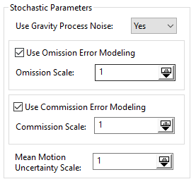
Propagator stochastic parameters panel
Instead of defining these properties in the Object Properties window, as in versions 7.10 of the ODTK software and earlier, they can now be defined directly in the propagator.
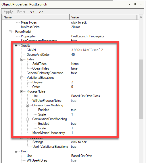
Satellite Force Model parameters
Updating the atmospheric model
Change the atmospheric model and update its parameters.
- Select Jacchia-Roberts in the component list.
- Click Delete (
 ).
). - Click New... (
 ).
). - Expand (
 ) Atmospheric Models when the New Function dialog box opens.
 - Select NRLMSISE 2000 ().
- Click to confirm your selection and to close the New Function dialog box.
- Note that the Use Stochastic Ballistic Coeff and Use Stochastic Density Correction check boxes are selected by default.
- Keep all the other values set to their defaults.
This is an empirical density model developed by the US Naval Research Laboratory and based on satellite data. It finds the total density by accounting for the contribution of N, N2, O, O2, He, Ar, and H number densities. It includes anomalous oxygen. This 2000 version has a valid range of 0 to 1,000 km.
This implements
Note that, as in the gravity model, the stochastic parameters of the atmospheric density model are now part of the propagator.
Updating the propagator numerical integrator
The
- Select the Numerical Integrator tab.
- Select the Use Fixed Step check box.
- Click to confirm your changes and to close the Propagator dialog box.
- Click to close the Component Browser.
The numerical integrator will now use the default 30-second integration steps.
Setting the ODTK satellite to use the new propagator
Now that you have configured your propagator, set the satellite to utilize it.
- Double-click on Launch2GEO () in the Object Browser to open the Object Properties window.
- Under Satellite - ForceModel - Propagator, select your new STK_ODTK_Tutorial propagator.
- Confirm that the Satellite - ForceModel - Gravity - DegreeAndOrder attribute is set to 40.
- Confirm that the Satellite - ForceModel - Drag - AtmDensityModel attribute is set to NRLMSISE 2000.
- Confirm that the Satellite - PropagatorControls - StepSize - StepControlMethod is set to Fixed.
- Confirm that the Satellite - PropagatorControls - StepSize - StepControlMethod is set to 0.5 min.
- Click in the Object Properties window to apply the property changes.
If you are using version 13.0 of the ODTK application to complete this tutorial, set the Satellite - ForceModel - UseComponentPropagator attribute to true.
Processing the post-launch measurements
You launch did not happen exactly as planned:
- The launch occurred five minutes later than panned.
- The burnout occurred at a slightly higher altitude than expected.
- At burnout, the spacecraft traveled a little faster than originally planned.
So, while the NominalMission Satellite object in the STK application still provides the general mission plan, it is no longer accurate enough to set the initial state in the ODTK application. You will begin the orbit determination process with an Initial Orbit Determination object and refining with a Least Squares object instead. You will then use the filter to compute the actual trajectory your satellite took.
Loading the post-launch tracking data
Add a tracking data file to be used in the orbit determination process. The observations were taken from your group of tracking stations and will be used in the orbit determination process to produce an estimate of the trajectory.
- Double-click on ODTK_STK (
 ) in the Object Browser to open its Properties.
 - Select the Scenario - Measurements - Files property.
- Click where indicated (click to edit) in the Value field.
- Click when the Scenario.Measurements.Files dialog box opens.
- Click where indicated in the Filename field.
- Navigate to <Install Dir>\Data\Resources\odtktraining\trackingdata.
- Select PostLaunch.geosc.
- Click .
- Click to confirm your selection and to close the Scenario.Measurements.Files dialog box.
- Click .
Previewing the measurements
Preview the measurements in the file to ensure they are correctly associated with the objects in this scenario.
- Right-click in the toolbar area.
- Select Default to show the Default toolbar if it is not already visible.
- Click Preview Measurements (
 ) in the Default toolbar.
 - Review the information in the Message Viewer.
You should see your four trackers and the Launch2GEO in the tracking data.
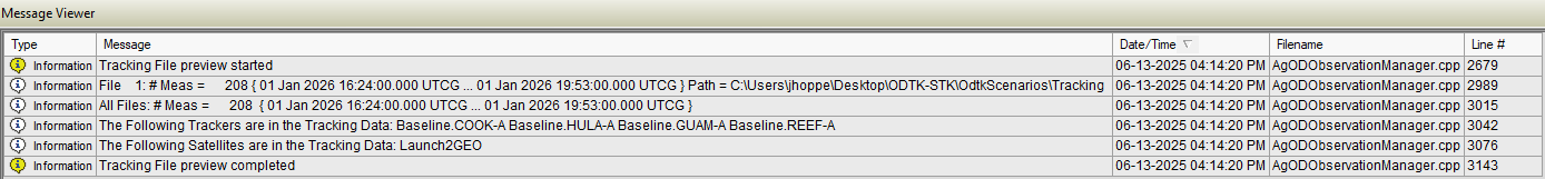
Tracking data preview
Generating a Measurement Times by Tracker report
Generate a report to show which tracker sees the satellite first.
- Select Static Product Builder (
 ) in the View menu.
 - Select the Outputs tab when the Static Product Builder window opens.
- Select the Measurement Times by Tracker graph style (
 ) from the Products Styles (Graphs and Reports) list.
 - Rename Data Product (
 ) Meas Times by Tracker by clicking its default name and entering the new one.
 - Click Run Selected (
 ) to launch the Graph Viewer window.
 - Review the graph.
![]()
Measurement Times by Tracker graph
HULA-A has the first set of available tracking measurements, so you will use that facility for further analysis.
Inserting an Initial Orbit Determination object
Add an
- Select Launch2GEO () in the Object Browser.
- Expand (
 ) the menu next to the Satellite object toolbar icon (
 ).
). - Select InitialOrbitDetermination (
 ).
). - Click .
Updating the Initial Orbit Determination object's properties
Confirm your method and select the tracking station facility to use for your IOD.
- Open InitialOrbitDetermination1's () Properties.
- Ensure that the InitialOrbitDetermination - Method property is set to HerrickGibbs.
- Set the InitialOrbitDetermination - SelectedFacility property to Facility/HULA-A.
- Click .
IOD methods are constructed to work with a specific mix of observation types. The Herrick-Gibbs IOD method uses three sets of range plus directions measurements to generate an initial orbit solution for a geocentric spacecraft. Since your tracking data contain azimuth, elevation, range and Doppler measurements.
Recall that HULA-A is the first facility to collect tracking data.
Selecting the observations from the tracking data
The Herrick-Gibbs IOD method enables you to select three observations from the tracking data. The ODTK application offers you a list of measurements to select from, which may span several orbit revolutions or several passes of tracking data. The Herrick Gibbs algorithm is valid for a selection that spans substantially less than one orbit period, and is typically applied to three measurements from the same tracking pass.
- Click where indicated in the Value field for the InitialOrbitDetermination - Method - SelectedMeasurements property.
- Click when the InitialOrbitDetermination.Method.SelectedMeasurements dialog box opens.
- Review the data in the Add Items(s) dialog box when it opens.
- Multi-select data points 0000, 0120, and 0240.
- Click to confirm your selections and to close the Add Item(s) dialog box.
- Click to close the InitialOrbitDetermination.Method.SelectedMeasurements dialog box.
- Click .
Each row in the Add Item(s) dialog box shows the time of available measurements (absolute and relative), the range in kilometers, and the elevation angle in degrees.
For Herrick-Gibbs, you want to select three measurements from the same pass, not a low elevation angle, and spaced a couple of minutes apart.
Performing the initial orbit determination
Run the Initial Orbit Determination tool and, if it converges and the Keplerian elements seem reasonable for a LEO orbit, copy them to the Launch2GEO Satellite.
- Ensure InitialOrbitDetermination1 () is selected in the Object Browser.
- Click Run (
 ) in the default toolbar.
 - Click Transfer to Satellite (
 ) to push the new initial state to the satellite.
 - Note the confirmation in the Message Viewer window.
Refining the initial state using Least Squares
At this point, you have generated an initial orbit solution directly from tracking measurements using the Herrick-Gibbs IOD method. Your goal is to progress to performing orbit determination using a sequential filter, but since IOD results often have large errors in them, you will further refine the initial state using the Least Squares process.
Inserting a Least Squares object
Add a
- Select Launch2GEO () in the Object Browser.
- Expand () the menu next to the IOD object toolbar icon (
 ).
). - Select LeastSquares (
 ).
). - Click .
Performing a least squares run
Run the Least Squares object and review its output. You can keep the default Stage duration of 4 hours, since you have tracking data for about 3.5 hours and want to process all of it.
- Select LeastSquares1 () in the Object Browser.
- Click Run ().
- Click Transfer to Satellite () to push the solution state to the initial state to the satellite.
- Note the details of the confirmation message in the Message Viewer window.
Transferring the least squares result to the parent satellite enables you to use the least squares result as the starting point for the filter.
Configuring an Optimal Sequential Filter
Add a
- Select ODTK_STK () in the Object Browser.
- Insert a Filter object (
 ).
). - Select the Filter object () in the Object Browser.
- Click Run ().
This will generate a .filrun file, which is the output of the filter.
Processing the measurements
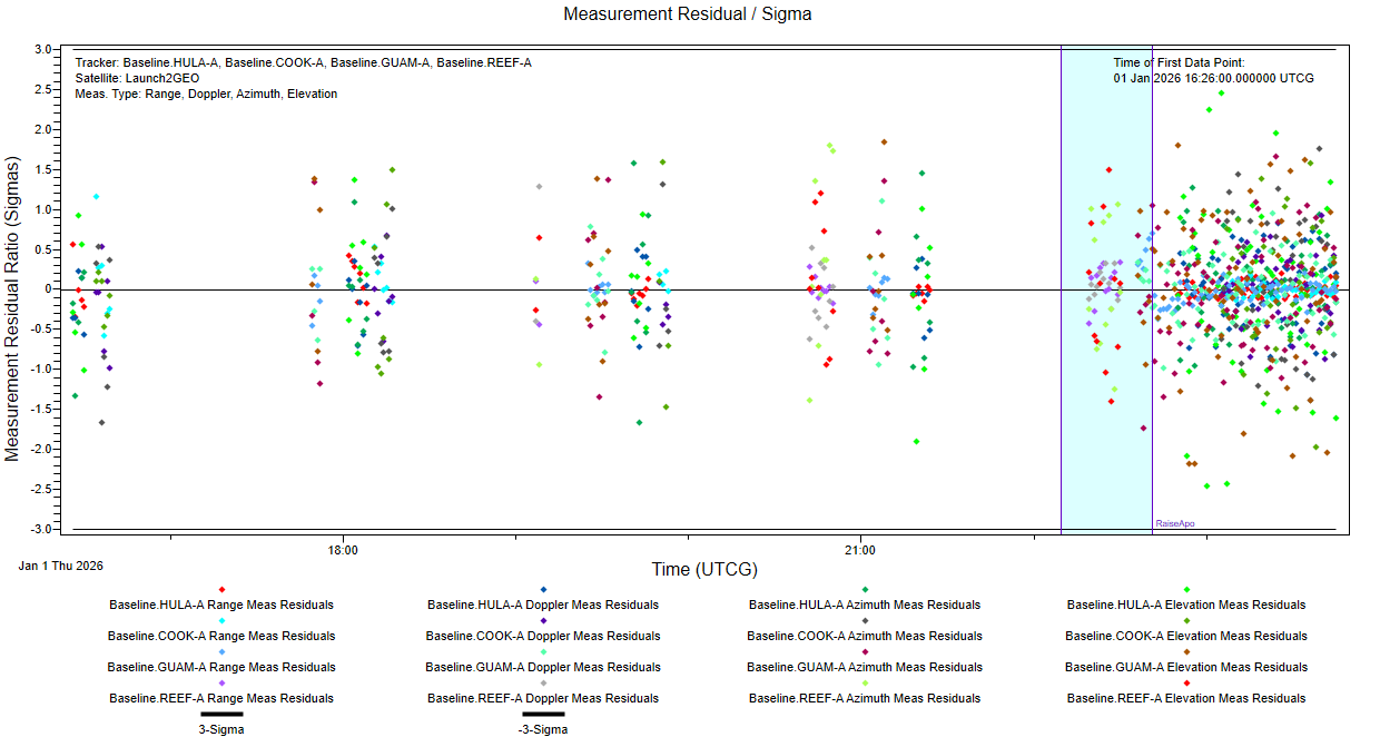
Create a Residual Ratios plot to make sure most measurements were accepted. A Residual Ratios plot displays normalized results, where the normalized residual is the residual divided by the measurement error root variance. Normalizing is useful to display residual behavior of two or more measurement types on one graph.
- Return to the Static Product Builder.
- Click Add Product (
 ).
). - Rename Data Product () Residual Ratios.
- Select Residual Ratios () graph style in the Product Styles (Graphs and Reports) list.
- Select the Inputs tab.
- Click .
- Click where indicated in the Objects field.
- Select Filter1 in the drop-down list.
- Click .
This will add the ODTK_STK.filrun file as the data source.
Creating the graph
With your data limited, run the graph.
- Click Run Selected ().
- Review the graph to make sure most measurements were accepted.
- Note the time of the last collected data points.
Not all measurements provided in tracking data files are used to update the estimation state during an estimation run. As an estimator (Filter or Least Squares) runs, it decides whether or not to accept a measurement and assign an appropriate
The last data were collected from COOK-A at 1 Jan 2026 19:53:00.000.
Your graph will look different than the one below, owing to when your
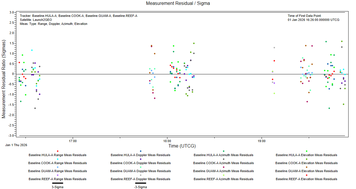
HULA-A Measurement Residual Ratio
Residual reports and graphs provide an indication of measurement quality and how well the solution matches the measurements. Another important result of orbit determination is the expected accuracy of the solution. The formal accuracy of an orbit determination solution is given by the state error covariance which is an output of the estimator along with the estimated state. The state error covariance is an n × n matrix, given a state size of n. While the covariance matrix as a whole is a lot of information to digest, the parts of it that indicate the positional accuracy of the solution are almost always of interest. When the filter is properly configured, the formal uncertainty, represented by the state error covariance matrix, is a reliable measure of orbit accuracy. The graph shows you measurements remain within the ±3-sigma bounds.
Creating and using flight dynamics records
While the propagator definition contains the various forces acting on the satellite, it does not include data at a specific epoch such as the state or its mass. This is where Flight Dynamics Records come in. A
Since the launch did not execute exactly as planned, you will use Astrogator to refine the maneuvers that get the satellite to the desired final orbit. To do that, Astrogator will need the best available state from the ODTK application. Use a Flight Dynamics Record to copy the orbit determined by the ODTK application to the STK application.
Creating a flight dynamics record in the ODTK application
You can create a new
- Select the Utilities menu.
- Select All Utilities....
- Double-click on Flight Dynamics Record Creator when the ODTK Utility Manager opens.
- Select Last Point in the Point Selection Mode drop-down list.
- Enter 1 Jan 2026 19:53:00.000 in the Pick Date field.
- Enter PostLaunch in the FD Record Name field.
- Click .
- Review the Status message.
- Save (
 ) your scenario.
This is the time of the last point of the tracking data.
The new FDR has been added to the Component Browser.
When you saved the scenario, the record was saved to the Flight_Dynamics subfolder of your scenario (for example., C:\Users\<username>\STK_ODTK 13\STK_ODTK\ODTK_STK\Flight_Dynamics\Flight_Dynamics_Records. You now need to get this over to STK application.
Exporting the flight dynamics record from the ODTK application
To avoid having to restart the STK application, export the FDR from the ODTK application.
- Select the Utilities menu.
- Select Component Browser....
- Select Postlaunch () in the Flight Dynamics Records List.
- Click Export File (
 ).
). - Navigate to your STK scenario folder (for example, C:\Users\<username>\STK_ODTK 13\STK_ODTK).
- Click .
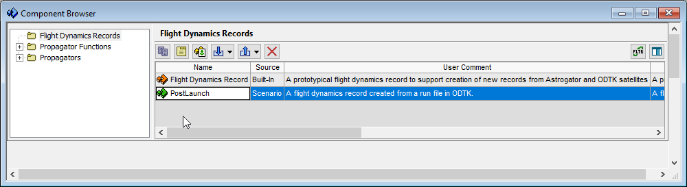
FDR in ODTK Component Browser
You can also add the PostLaunch FDR to your user collection by clicking Add to Collection (![]() ) to make it available in other scenarios. This will copy it into a folder from which both the STK and ODTK applications load files at start up. However, this will require you to restart the STK application to access the component.
) to make it available in other scenarios. This will copy it into a folder from which both the STK and ODTK applications load files at start up. However, this will require you to restart the STK application to access the component.
Importing the flight dynamics record into the STK application
With you FDR created, import it for use in the STK application.
- Return to the STK application ().
- Select the Utilities menu.
- Select Component Browser... (
 ).
). - Select the Flight Dynamics Records () folder in the Select Component Type list.
- Click Import File (
 ).
). - Select PostLaunch.FlightDynamicsRecord.
- Click to confirm your selection and to import the FDR.
- Select the Propagators () folder.
- Click to close the Component Browser.
Note that the STK ODTK Tutorial propagator was also transferred as part of the Flight Dynamics Record.
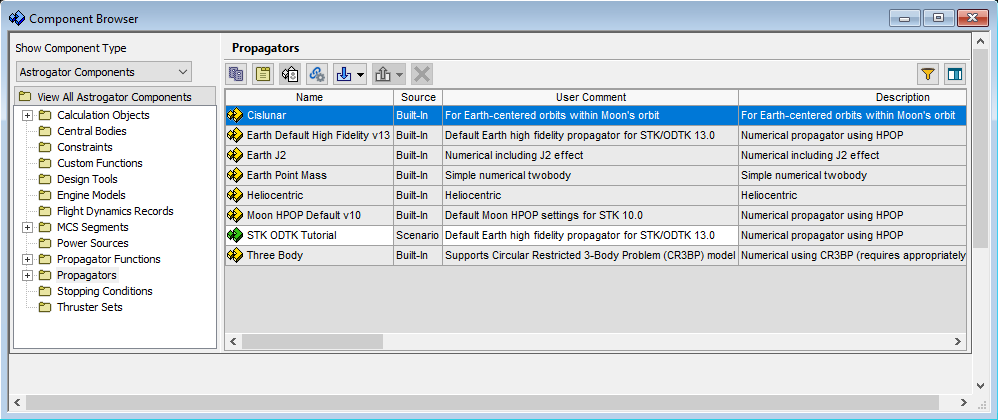
STK ODTK Tutorial propagator in STK Component Browser
Setting the initial state of PostLaunch satellite with the flight dynamics record
You can use the
- Right-click on Postlaunch () in the Object Browser.
- Select Properties ().
- Ensure the Initial State (
 ) segment is selected in the MCS.
 - Click on the Basic - Orbit page when the Properties Browser opens.
- Select Flight Dynamics Record in the Source Type drop-down list in the New Vector Source panel when the Initial State Import Tool dialog box opens.
- Click the ellipsis (
 ) next to the Flight dynamics record field.
 - Select PostLaunch () when the Select Component dialog box opens.
- Click to confirm your selection and to close the Select Component dialog box.
- Click in the Results panel.
- Click to apply the new initial state vector to the Initial State sequence.
Note that the MCS of the PostLaunch satellite is almost identical to that of the NominalMission satellite, with the exception that it starts from an Initial State segment instead of a Launch.
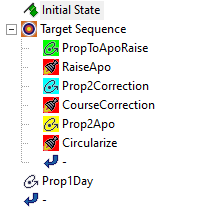
PostLaunch MCS
This will generate a new initial state vector. The results will appear in the Results panel.
This will set the initial state of the satellite and load the propagator but will not apply the propagator to all Propagate and Finite maneuver segments. Note that the Initial State's orbit epoch has been set to 1 Jan 2026 19:53:00.000 UTCG. Recall that this is the time of the last point of the tracking data that you set when you created the FDR.
Applying the new propagator to all MCS segments
While you loaded the STK ODTK Tutorial propagator into the STK application, it is not being used by the MCS components of the PostLaunch satellite.
- Click Configure MCS Segment Propagators (
 ) in the MCS toolbar.
 - Ensure the Replace All Propagators option is selected when the Configure MCS propagator dialog box opens.
- Click the ellipsis () next to the Replace with this propagator field.
- Select STK ODTK Tutorial () when the Select Component dialog box opens.
- Click .
- Click to select all the MCS segments.
- Click .
- Click to confirm your changes and to close the Configure MCS propagator dialog box.
Viewing the stochastic parameters
Review the Initial State segment’s stochastic parameters.
- Select the Stochastic Parameters tab.
- Note the values.
Your values will be different than the ones shown below.
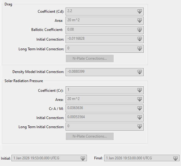
PostLaunch stochastic parameters
Since you set the initial state from a Flight Dynamics Record, the values are grayed out and Astrogator will use the corrections to the drag and SRP estimates from the ODTK application. The corrections will decay from their initial values at a rate specified by the respective half life value from the propagator. Unlocking the initial state would allow us to overwrite these values.
Propagating the PostLaunch satellite
Propagate the PostLaunch satellite.
- Select the check box for PostLaunch () in the Object Browser.
- Click Run Entire Mission Control Sequence (
 ).
). - Click Clear Graphics (
 ) to remove the iterations.
 - Bring the 3D Graphics window to the front.
- Increase the animation Time Step (
 ) to 60.00 sec.
 - Click Start (
 ) to view the propagated orbits.
 - Click Reset (
 ) when finished.
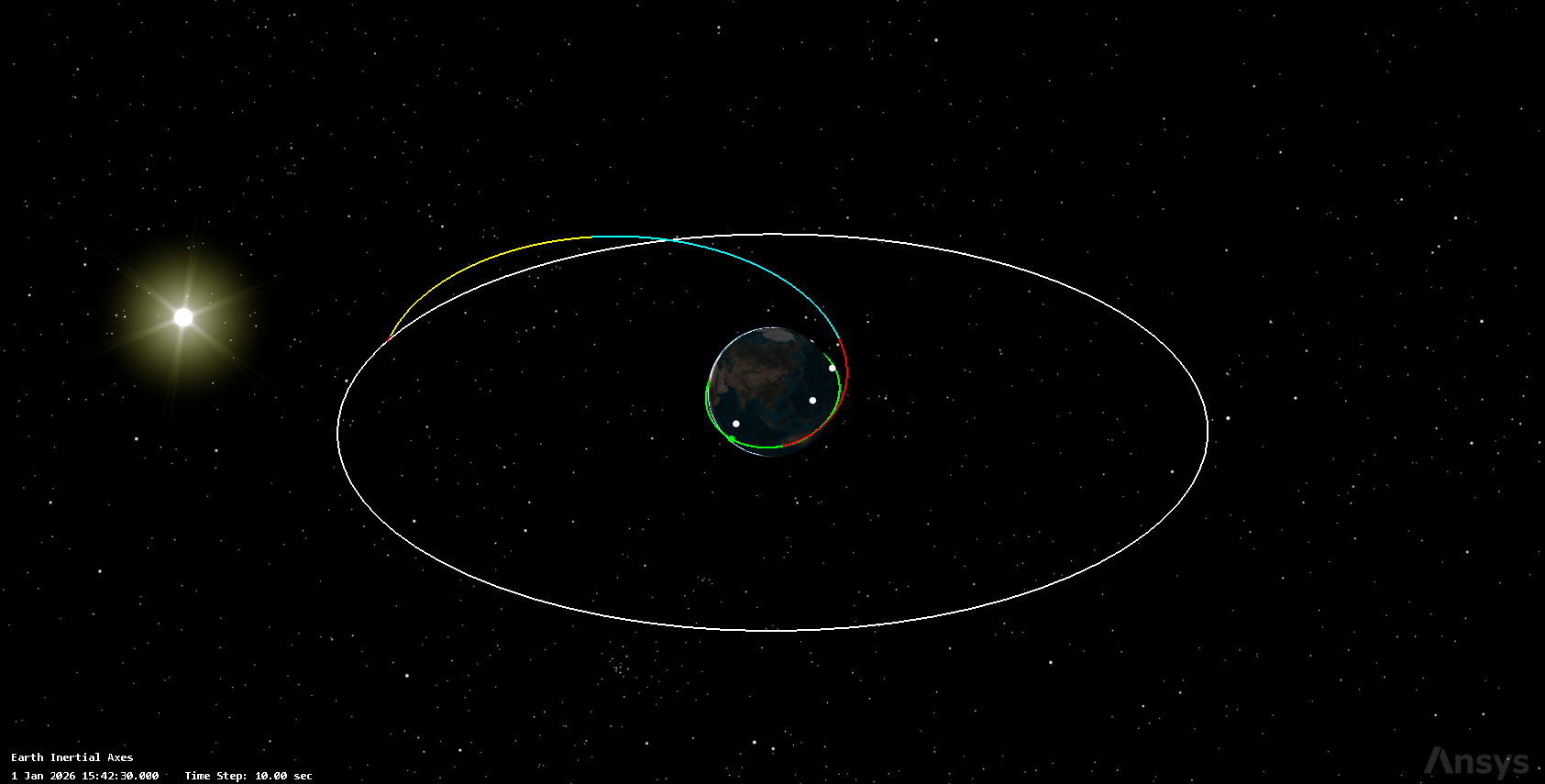
You want to visualize the orbit of the satellite as it was launched compared to that of the NominalMission satellite.
If it does not converge in the allowed number of iterations, click Run Entire Mission Control Sequence again until all solutions converge.
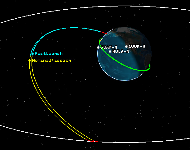
PostLaunch and NominalMission orbits
Updating the ODTK application with an acceleration history file
The Astrogator capability computed the required maneuvers to complete the mission starting with the launch errors. These are the updated maneuvers you will command the satellite to perform. Once they executed by the satellite, and you receive new post-maneuver tracking data, you have to transfer the updated maneuvers into the ODTK application as well. You can transfer the newly updated maneuver details from the STK application to the ODTK application by creating acceleration history files.
Creating a custom acceleration history report
You can use an
- Right-click on PostLaunch () in the Object Browser.
- Select Report & Graph Manager... (
 ) in the shortcut menu.
 - Select the My Styles () folder.
- Click Create a new report style (
 ) in the Styles toolbar.
 - Name the new report Accel Hist.
- Select the Enter Key.
- Expand () the Astrogator Accel Hist () data provider when the Report Style window opens.
- Select the
 ) data provider element.
 - Insert (
 ) Accel Hist into the Report Contents list.
 - Click to confirm your selection and to close the Report Style window.
The STK application comes with two preinstalled report styles:
Creating a custom acceleration history report
With your data provider element selected, generate the report and review the contents of the acceleration history file.
- Select the Accel Hist (
 ) report.
 - Click .
- Note that the report itself contains a summary of files that STK generated.
- Close the Accel Hist report.
- Navigate to the location of your generated acceleration history files in Windows Explorer.
- Select PostLaunch.Target_Sequence.RaiseApo.accelhist.
- Open PostLaunch.Target_Sequence.RaiseApo.accelhist with a text editor of your choice.
- Inspect its contents.
This Generates an acceleration history file for each finite maneuver segment of the Astrogator satellite. The name of each file reflects the maneuver segment name and the name of any associated target sequence. The STK application places the files in a folder called AccelHist within the scenario directory. It also creates an additional file, AllAccelHist.accelhist, that gather all the acceleration data of the separate files.
Acceleration history files contain the acceleration due to the maneuver over time. Since you have only refined the RaiseApo maneuver so far, skip the Circularize acceleration history file for now.
The file data consists of five columns: Time, ACCELx, ACCELy, ACCELz, and MassChangeRate. The format of the file is compatible for ingestion by the ODTK application. Note that the acceleration history file table contains some common elements called keywords. Keywords and their associated values (except END) must precede the specification of the data and the actual data points.
Creating a finite maneuver in the ODTK application with the acceleration history file
Back in the ODTK application, add a
- Return to the ODTK application ().
- Open Launch2GEO's () Properties.
- Scroll to the Satellite - Forcemodel - FiniteManeuvers property.
- Click where indicated.
- Click when the Satellite.Forcemodel.FiniteManeuvers dialog box opens.
- Select FiniteManAccelFile when the Add Item(s) dialog box opens.
- Click to confirm your selection and to close the Add Item(s) dialog box.
- Set the following values:
- Click to confirm your changes and to close the Satellite.Forcemodel.FiniteManeuvers dialog box.
- Click .
| Name | Value1 |
|---|---|
| Name | RaiseApo |
| AccelHistoryFilename | C:\Users\<username>\Documents\STK_ODTK 13\STK_ODTK\AccelHist\PostLaunch.Target_Sequence_RaiseApo.accelhist |
| Estimate | MagnitudeOnly |
| Mass - Isp | 300 sec (to match the engine model in Astrogator) |
| Uncertainty - PercentMagnitudeSigma | 5% |
Calibrating the engine component
While you now know the corrected desired maneuver, there will be errors due to the actual engine not being calibrated yet. By processing the PostDV1 measurement file, the ODTK software can estimate corrections to the planned maneuvers, which will allow you to calibrate the spacecraft's engine just in time for the 2nd maneuver.
Loading the new measurements
Load the PostDV1.geosc file while keeping PostLaunch.geosc enabled.
- Open ODTK_STK's () Properties.
- Click to edit the Scenario - Measurements - Files property.
- Click .
- Click where indicated in the new entry.
- Navigate to <Install Dir>\Data\Resources\odtktraining\trackingdata.
- Select PostDV1.geosc.
- Click .
- Click to confirm your selection and to close the Scenario.Measurements.Files dialog box.
- Click .
Processing the PostDV1 measurements
Re-run your filter and review the data.
- Select Filter1 () in the Object Browser.
- Run () the filter.
- Return to your Residual Ratios plot.
- Refresh (
 ) the graph.
 - Review the graph to see if most of the measurements were accepted (that is, fall within the ±3-sigma bounds).
The ODTK application processes maneuvers in the filter after processing all measurements (if any) during the maneuver time.
Your graph will look different than the one shown below.
Residual Ratios plot with postDV1 tracking data
Creating a Finite Maneuver Thrust Magnitude Percent graph
Create a new data product to show the magnitude of the thrust correction of the RaiseApo maneuver by copying your existing Residual Ratios data product.
- Return to the Static Product Builder.
- Select Residual Ratios () in the Product List.
- Click Copy Product (
 ).
). - Rename Copy_of_Residual Ratios () Thrust Magnitude Pct.
- Select the Outputs tab.
- Select Finite Mnvr Thrust Magnitude Pct () in the Product Styles (Graphs and Reports) list.
- Run () the selected data product.
- Review the graph.
The Finite Mnvr Thrust Magnitude Pct data product displays estimated thrust magnitude correction as a percentage of a the nominal thrust during a finite maneuver.
Your graph may look slightly different than the one below.
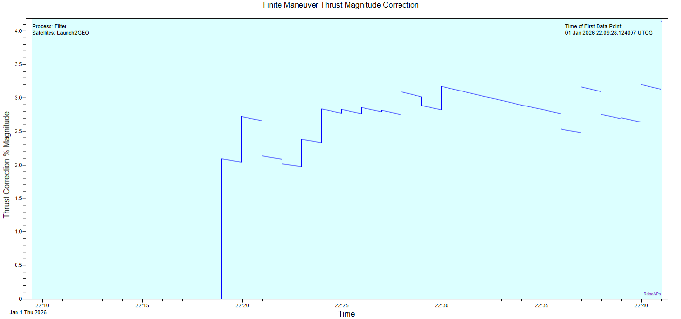
Finite Thrust Maneuver Magnitude Correction graph
Since the engine was not yet calibrated, there were some inaccuracies. In this case, the engine provided slightly more thrust than expected. The average correction over the entire maneuver is about 2%.
Creating a calibrated engine component in the STK application
Create an
- Return to the STK application ().
- Return to the Component Browser ().
- Select the Engine Models () folder in the Select Component Type list.
- Select the Constant Thrust and Isp () component in the Engine Model list.
- Click Duplicate component ().
- Enter 102% in the Name field when the Field Editor dialog box opens.
- Click .
- View 102%'s () Properties ().
- Set the Thrust to 510 N when the 102% dialog box opens.
- Click to confirm your changes and to close the 102% dialog box.
Performing the final maneuver estimation
Now that you have a better idea of how your engine performs, go through the above process one more time to get a corrected circularization maneuver. Unfortunately, due to the launch and engine calibration error, you now need to perform a small course correction maneuver as well. Use the PostDV1 satellite to get your final maneuver estimates in the STK application.
Transferring the latest state from the ODTK application into the STK application
Create a new flight dynamics record in the ODTK application from the latest tracking data and transfer it to the STK application.
- Return to the ODTK application ().
- Open the Flight Dynamics Record Creator from the Utility.
- Create a new FDR for the Launch2GEO satellite named PostDV1 at the last point processed by the filter, which should be on 1 Jan 2026 23:44:58.194.
- Add the FDR to the ODTK Component Browser.
- Export the PostDV1 flight dynamics record from the Component Browser to the STK_ODTK STK scenario folder.
- Return to the STK application ().
- Open the PostDV1 () satellite's Properties ().
- Open the Component Browser () from the MCS toolbar.
- Import () PostDV1.FlightDynamicsRecord into the Flight Dynamics Records () folder.
- Close the Component Browser.
Updating PostDV1's initial state
Update PostDV1's initial state segment with the PostDV1 FDR.
- Select the Initial State () segment in the MCS.
- Click .
- Select Flight Dynamics Record in the Source Type drop-down list in the New Vector Source panel when the Initial State Import Tool dialog box opens.
- Click the ellipsis () next to the Flight dynamics record field.
- Select PostDV1 () when the Select Component dialog box opens.
- Click to confirm your selection and to close the Select Component dialog box.
- Click in the Results panel.
- Click to apply the new initial state vector to the Initial State sequence.
- Click .
Note that the orbit epoch of the initial state has been set to 1 Jan 2026 23:44:58.194, the point last processed by the filter that you chose for the FDR.
Configuring PostDV1's propagators
Configure the propagator for PostDV1's Maneuver and Propagate segments.
- Click Configure MCS Segment Propagators () in the MCS toolbar.
- Select all the segments in the Segment Properties list.
- Replace all propagators with the STK ODTK Tutorial () propagator.
- Apply the propagator and integrator to the selected segments.
- Click .
- Click .
Updating PostDV1's CourseCorrection Manuever segment
Update the CourseCorrection Maneuver segment to use the calibrated 102% engine model you created earlier for both the Finite and Impulsive maneuver types.
- Select the CourseCorrection () Maneuver segment in the MCS.
- Select the Engine tab.
- Ensure the Maneuver Type is set to Finite.
- Click the ellipsis () next to the Engine Model option in the Propulsion Type panel.
- Select 102% () when the Select Component dialog box opens.
- Click to confirm your selection and to close the Select Component dialog box.
- Select Impulsive in the Maneuver Type drop-drop list.
- Select the 102% () engine model component for the Impulsive maneuver type.
Updating PostDV1's Circularize Maneuver segment
Update the Circularize Maneuver segment to use the calibrated 102% engine model you created earlier.
- Select the Circularize () Maneuver segment in the MCS.
- Set the segment to use the 102% () engine model for the Finite Maneuver type.
- Change the Maneuver Type to Impulsive.
- Select the 102% () engine model component for the Impulsive maneuver.
- Click to confirm your changes and to keep the Property Browser open.
The Astrogator capability computes the impulsive maneuver first, since it converges easier. Using the results from that analysis, it will compute the initial guesses for a finite maneuver and then use those to develop a solution. By setting the engine model for both maneuver types to use your custom 102% engine model, you ensure that both solutions will have accurate results.
Propagating the satellite and generating new acceleration history files
Propagate the PostDV1 satellite and generate new acceleration history files for the CourseCorrection and the Circularize maneuvers.
- Select the check box for PostDV1 () in the Object Browser.
- Run () the entire MCS.
- Clear the graphics () of the iterations.
- Review the propagated orbit in the 3D Graphics window.
- Right-click on PostDV1 () in the Object Browser.
- Select Report & Graph Manager... () in the shortcut menu.
- Generate an Accel Hist () report.
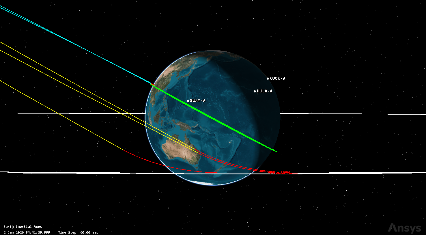
Course Correction and circularization maneuvers
Generating an Accel Hist report will also generate acceleration history files for both the Course Correction (PostDV1.Target_Sequence.CourseCorrection.accelhist) and Circularize (PostDV1.Target_Sequence.Circularize.accelhist) maneuvers.
Performing a final ODTK run
Now that you know what maneuvers were executed by the satellite, you can add them to the ODTK scenario. Add the two finite maneuvers to the Satellite in the ODTK application.
- Return to the ODTK application ().
- Open Launch2GEO's () Properties.
- Add a new Finite maneuver of the FiniteManAccelFile type representing the Course Correction maneuver to the satellite, being sure to keep the RaiseApo maneuver you created earlier.
- Set the following values:
- Add another new Finite maneuver of the FiniteManAccelFile type representing the circularization maneuver, being sure to keep the two maneuvers you created earlier.
- Set the following values:
- Click .
- Click .
| Name | Value1 |
|---|---|
| Name | CourseCorrection |
| AccelHistoryFilename | C:\Users\<username>\Documents\STK_ODTK 13\STK_ODTK\AccelHist\PostDV1.Target_Sequence.CourseCorrection.accelhist |
| Estimate | MagnitudeOnly |
| Mass - Isp | 300 sec |
| Uncertainty - PercentMagnitudeSigma | 5% |
| Name | Value1 |
|---|---|
| Name | Circularize |
| AccelHistoryFilename | C:\Users\<username>\Documents\STK_ODTK 13\STK_ODTK\AccelHist\PostDV1.Target_Sequence.Circularize.accelhist |
| Estimate | MagnitudeOnly |
| Mass - Isp | 300 sec |
| Uncertainty - PercentMagnitudeSigma | 5% |
Loading the final tracking file
Load the final tracking file into the scenario while keeping both PostLaunch.geosc and PostDV1.geosc enabled.
- Open ODTK_STK's () Properties.
- Click to edit the Scenario - Measurements - Files property.
- Click .
- Click where indicated in the new entry.
- Navigate to <Install Dir>\Data\Resources\odtktraining\trackingdata.
- Select PostDV2.geosc.
- Click .
- Click to confirm your selection and to close the Scenario.Measurements.Files dialog box.
- Click .
Processing the PostDV2 measurements
Now that your satellite has performed the recalculated maneuvers needed to bring it into your desired orbit, confirm that it has reached your goal by processing the post-DV2 tracking measurements.
Refreshing your Residual Ratios plot
Re-run your filter and review the data.
- Select Filter1 () in the Object Browser.
- Run () the filter.
- Return to your Residual Ratios plot.
- Refresh () the graph.
- Review the graph to see if most measurements were accepted.
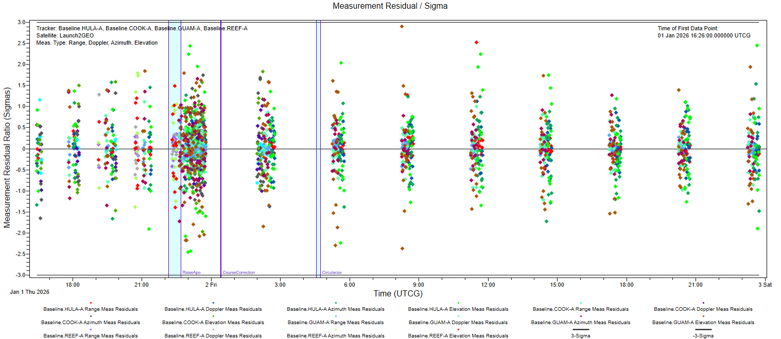
Residual Ratios plot with PostDV2 tracking data
You can now see all three maneuvers on your residuals graph. The graph shows that the updated measurements still remain within the ±3-sigma bounds.
Adding a Smoother
The ODTK software has two smoothing algorithms. One is a forward-running variable time lag sequential smoother that runs with the filter and is a child of the filter object. This algorithm is called the variable lag smoother (VLS). The VLS is essentially a series of fixed-epoch smoothers (FES) at selected filter epochs. Each FES serves to map measurement information, as measurements are processed backward in time, to update the trajectory at its specific epoch. While a VLS provides the most complete smoothed trajectory possible at each step of the filter run, because it runs simultaneously with the filter, it will extend the filter run times. For example, a VLS may be preferable to improve orbit knowledge at the end of a maneuver or other critical point in time for a space mission. But due to increased run time, you may not want to run at every time and measurement update.
The second smoother type is a backward-running fixed-interval smoother (FIS), which runs after the filter is completed. It requires the filter to provide data to the smoother via a set of "rough" file(s). The ODTK software's smoothing algorithm runs backward in time, starting at the end of the filter run and maps information backward. The trajectory produced by the smoother has all measurement information represented at all times. It is common for an OD analyst to work with both estimation tools in a complimentary manner.
Because a FIS smoother runs much faster, you will add the FIS smoother to the scenario instead of the VLS.
Generating "rough" data from the filter
To employ the FIS, you need to turn on the generation of a "rough" file from the filter. The "rough" file is output during the filter run and contains all inputs needed by the smoother.
- Select Filter1 () in the Object Browser.
- Double-click it to open its Properties.
- Set the Filter - Output - SmootherData - Generate attribute to true.
- Click .
- Select Filter1 () in the Object Browser.
- Run () the filter.
This last action exposes the Filter - Output - SmootherData – Filename attribute. This option is the name of the .rough file that is used to pass data from the filter to the FIS smoother.
This will now generate a .rough file in addition to the .filrun file it generated early.
Creating a Smoother object
The FIS smoother is enabled by inserting a Smoother object into the scenario.
- Select ODTK_STK () in the Object Browser.
- Insert a Smoother (
 ) object.
Loading the filter output into the smoother
The inputs for the fixed-interval smoother are in the "rough" file generated by the filter, so you need to associate the "rough" file with your new smoother object.
- Double-click on Smoother1 () in the Object Browser to open its Properties.
- Click on the Smoother - Input - Files value field.
- Click when the Smoother.Input.Files dialog box opens.
- Load the ODTK_STK_Filter1.rough file that was generated when you last ran the filter.
- Click to close the Smoother.Input.Files dialog box.
- Set the Smoother - Output - FilterDifferencingControls – Generate attribute to true. This will enable you to check your filter and smoother for consistency later.
- Click .
- Select the Smoother object () in the Object Browser.
- Run () the smoother.
This will generate a .smtrun file and a .difrun file for use by the Static Product Builder Reporting and Graphing interface.
Generating a Position Uncertainty plot
Generate a Position Uncertainty plot. This graph displays the 2-sigma position uncertainty in radial, in-track, and cross-track components, taken from the covariance.
- Return to the Static Product Builder.
- Click Add Product ().
- Rename Data Product (
 ) Pos Uncertainty.
 - In the Outputs tab, select Position Uncertainty () in the Product Styles (Graphs and Reports) list.
- Select the Inputs tab.
- Click in the Data Source panel.
- Click to edit the Objects.
- Select Smoother1-smtrun in the drop-down list.
- Run () the selected data product to review the results.
Your graph will look different than the one shown below.
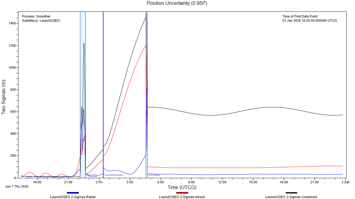
Position Uncertainty Plot
The smoother starts at the right side of the graph with the final uncertainty from the filter then moves backwards in time. Note the reduction in the uncertainty early in the estimation time span that the smoother provides. This is due to the mapping of information from later observations back to earlier times. The output from the filter is discontinuous where measurements have been processed, but these jumps are removed by the smoother. The smoother output is therefore what is labeled as the definitive orbit solution for use in subsequent analyses.
Generating a Position Consistency plot
Now that you’ve run both the filter and smoother, you can perform quality checks on your solution. A simple quality check to perform is the Position Consistency check. This check will test to see if the difference between the filter and smoother solutions is consistent with the covariance on that difference. The test is typically applied to individual elements of the state, in which case the test statistic should remain with ±3 sigma on 99% of the points sampled.
- Return to the Static Product Builder.
- Select Pos Uncertainty () in the Products list.
- Click Copy Product ().
- Rename Copy_of_Pos Uncertainty () Pos Consistency.
- Change the Input to use the ODTK_STK.difrun file.
- Select the Outputs tab.
- Select Pos Consistency () in the Product Styles (Graphs and Reports) list.
- Run () the selected data product.
- Review the results.
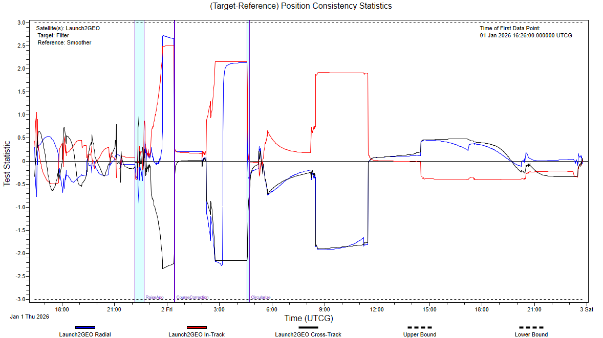
Position Consistency Plot
Creating a Measurement Summary by Altitude plot
Finally, generate a Measurement Summary by Altitude graph to confirm that your satellite has settled into its targeted GEO orbit following the Hohmann transfer.
- Return to the Static Product Builder.
- Select Pos Uncertainty () in the Products list.
- Click Copy Product ().
- Rename Copy_of_Pos Uncertainty () Meas Sum by Alt.
- Select Measurement Summary by Altitude () in the Product Styles (Graphs and Reports) list.
- Run () the selected data product.
- Review the results.
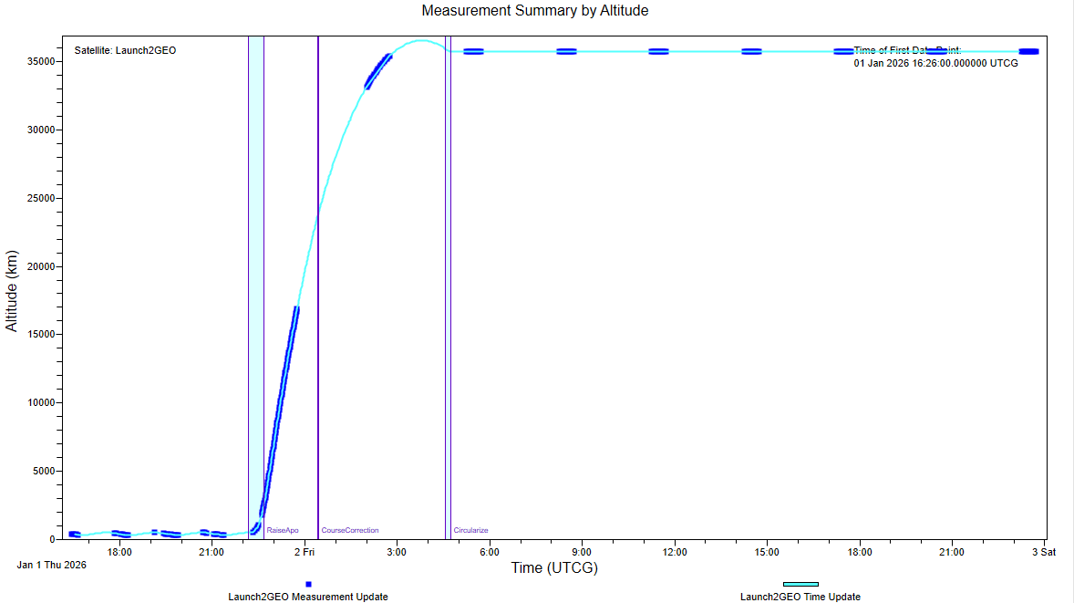
Measurement Summary by Altitude plot
The smoothed measurements show the satellite's altitude rapidly increasing after the maneuver to raise the apoapsis was performed. Subsequent tracking data confirm that your satellite settled into an orbit at approximately 35,776 km, 10 km below GEO altitude, as you had originally planned, following the course correction maneuver and the maneuver to circularize the orbit.
By using the ODTK and STK applications in conjunction with one another, you not only planned your mission, you analyzed and modified it as it unfolded using the latest available data. By further processing the tracking data, you confirmed that the mission's goals were met.
Saving your work
Clean up your workspaces and save your work.
- Close any open reports, properties and tools.
- Save () your work.
- Close the STK application.
- Return to the ODTK application ().
- Return to the Static Product Builder.
- Click Save As (
 ) below the Products list.
 - Enter STK_ODTK in the name field when the Save As dialog box opens.
- Click to save your ODTK data product list and to close the Save As dialog box.
- Save () your work.
- Close the ODTK application.
Summary
You used the ODTK application to process the orbital measurements of a satellite whose launch did not go according to the mission plan you developed using the STK application's Astrogator capability. After processing the measurements to get an accurate model of its state, you created a flight dynamics record of full state of the satellite to feed back into the STK application. You used the flight dynamics record to compute the updated maneuvers needed to achieve your desired orbit. You exported an acceleration history file from the results and imported it into the ODTK application to estimate corrections to the planned maneuvers with another flight dynamics record. You calibrated your engine model in the STK application based on these measurements. You modeled the corrected maneuvers using the Astrogator capability and exported another acceleration history file to the ODTK application to account for the maneuvers, and analyzed the resulting state of the satellite using post-maneuever tracking measurements to confirm your mission was now proceeding as intended.