STK Premium (Space) or STK Enterprise
You can obtain the necessary licenses for this tutorial by contacting AGI Support at support@agi.com or 1-800-924-7244.
The results of the tutorial may vary depending on the user settings and data enabled (online operations, terrain server, dynamic Earth data, etc.). It is acceptable to have different results.
Capabilities covered
This lesson covers the following capabilities of the Ansys Systems Tool Kit® (STK®) digital mission engineering software:
- STK Pro
- STK SatPro
Problem statement
Due to its elliptical orbit around the Sun, the Earth does not consistently receive solar rays of the same strength from month to month, or even day to day. The same applies to satellites. You need to perform long-term analysis of the potential power generation on board a satellite to understand how it will change throughout the year. This information will help you predict your power budget moving forward.
Solution
Use the SatPro capability to perform power analysis on a satellite using the Solar Panel tool. You will analyze changes in its power generation over an entire year, with a focus on the changes in power that occur when the Sun is closest to and farthest from the Earth during that year (the times of perihelion and aphelion, respectively).
What you will learn
Upon completion of this tutorial, you will be able to:
- Load satellite models registered for solar panel analysis into the STK application
- Use the Solar Panel tool to perform power analysis
- Create reports and graphs from the data generated by the Solar Panel tool
Video guidance
Watch the following video. Then follow the steps below, which incorporate the systems and missions you work on (sample inputs provided).
Creating a new scenario
First, create a new STK scenario, then build from there.
- Launch the STK (
 ) application.
 - Click
 Create a Scenario in the Welcome to STK dialog box.
 - Enter the following in the New Scenario Wizard:
- Click when you finish.
- Click Save (
 ) when the scenario loads. A folder with the same name as your scenario is created for you.
 - Verify the scenario name and location shown in the Save As dialog box.
- Click .
| Option | Value |
|---|---|
| Name | Seasonal_Power |
| Location | Default |
| Start | 21 Dec 2016 00:00:00.000 UTCG |
| End | + 366 days |
Modeling the Aqua satellite
You will model the NASA Earth science satellite Aqua (EOS-PM-1) in this scenario. It was launched in 2002. Designed to last six years, by December, 2016, it had well surpassed its design life; yet, it was still doing useful work in space, and a significant power generation margin remained. Since the satellite was still used, engineers and operators wanted to optimize the efficiency operations performed by the vehicle and its on-board equipment. You are interested in its potential for power generation over the course of a single solar cycle, beginning with the winter solstice of 2016, occurring on December 21, 2016, and ending on the following winter solstice on December 21, 2017.
Inserting Aqua from the Standard Object Database
Use the Aqua model from the Standard Object Database, which has its on-board equipment already configured. This will save you some scenario building time.
- Bring the Insert STK Objects (
 ) tool to the front.
 - Insert a Satellite (
 ) object using the From Standard Object Database (
 ) method.
 - Click .
- Enter Aqua in the Name or ID field when the Search Standard Object Data dialog box opens.
- Click .
- Select the Result with Space Surveillance Catalog Number of 27424, whose Data Source is AGI's Standard Object Data Service.
- Click .
- Click to close the Search Standard Object Data dialog box.
This will insert the Aqua satellite and an attached Sensor (![]() ) object, Aqua_Modis_Vis_Ir_FixedPt_FieldOfView.
) object, Aqua_Modis_Vis_Ir_FixedPt_FieldOfView.
Changing your perspective
Reposition your view so that you can get a better look at Aqua’s solar panels in the 3D Graphics window.
- Bring the 3D Graphics window to the front.
- Right-click on Aqua_27424 () in the Object Browser.
- Select Zoom To in the shortcut menu.
- Use your mouse to adjust the perspective to view the satellite.
This will set the satellite as the focal point in the 3D Graphics window.
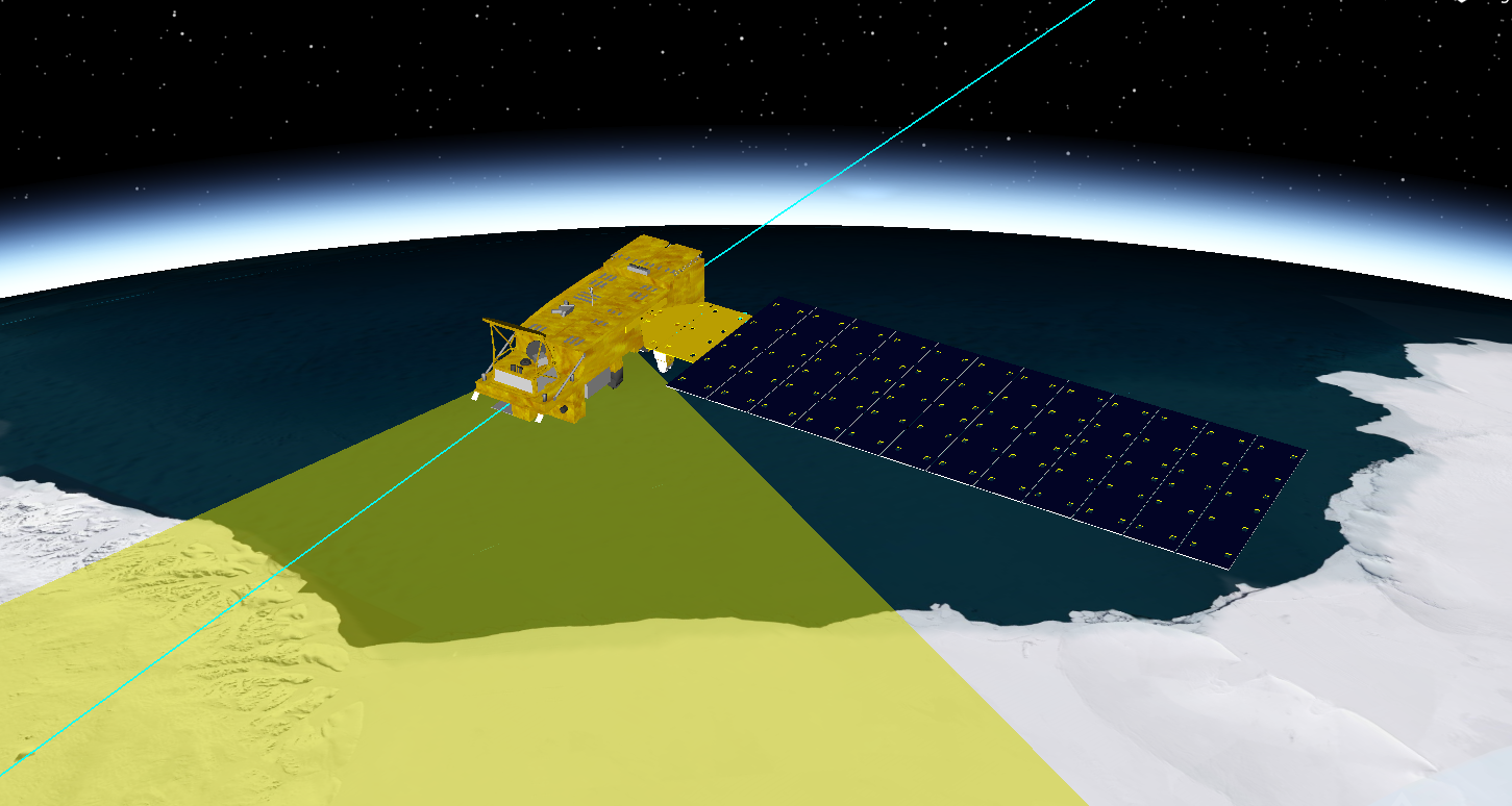
3D Graphics view of the Aqua Satellite
Viewing Aqua in the Solar Panel tool
The
Opening the Solar Panel tool
Open the Solar Panel tool to view the available solar panels on the Aqua satellite.
- Right-click on Aqua_27424 () in the Object Browser.
- Select Satellite in the shortcut menu.
- Select Solar Panel... in the Satellite submenu.
Viewing the solar panels in the Solar Panel View window
The
- Bring the Solar Panel View window to the front when the Solar Panel tool opens.
- Now bring the Solar Panel tool to the front again.
- Review the Solar Panel Groups list in the Visualization panel.
- Click to Close the Solar Panel tool.
- Close (
 ) the Solar Panel View window.

Solar Panel View of Aqua
Note the entire satellite is entirely black, with no obvious solar panels indicated.
Note there are no solar panel groups listed on the Solar Panel tool for Aqua. This is because they are not defined in the current model file. You will have to use another model file that contains a definition of the solar panel groups.
Using a model with defined solar panels
For solar panel groups to show up in the Solar Panel Groups list, and thus be useable by the Solar Panel tool, they must be defined in the object's model.
Changing Aqua’s model
Right now, Aqua is set to use the default catalog model file, aqua.glb, which is a glTF model file. Switch out that model file for a customized model file, which is included with your STK software install, by updating the Satellite object's
- Open Aqua_27424’s () Properties (
 ).
). - Select the 3D Graphics - Model page.
- Click the ellipsis button (
 ) beside the Model File option in the Model panel.
 - Go to <Install Dir>\Data\Resources\stktraining\samples when the File dialog box opens.
- Select the aquaSPGroups.mdl file.
- Click to use the aquaSPGroups.mdl file in your scenario and to close the File dialog box.
- Click to confirm your changes and to keep the Properties Browser open.
This is an
Viewing the solar panel groups in the model file
You can also determine if the model file has solar panel groups by examining the model file itself. If the solar panel groups are defined as a component, you will see them defined in the
- Navigate to <Install Dir>\Data\Resources\stktraining\samples in Windows File Explorer.
- Open the aquaSPGroups.mdl file in a text editor of your choice (for example, Windows Notepad or Notepad++).
- Scroll to the
SolarPanel groupssection. - Note the syntax of the entries, for example,
SolarPanelGroup SlrPnl1 14.0. - Once you are done examining the model file, close the text editor.
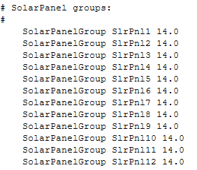
Solar Panel Groups in model file
Just like the real Aqua satellite, the Aqua model is equipped with 12 solar arrays. Each array is defined as a group in the satellite model file. Having several individual arrays enables you to articulate the solar panels individually, rather than articulating one huge "solar panel wing."
The SolarPanelGroup parameter specifies the name of the solar panel group and the efficiency of the solar panel used in solar panel calculations. Multiple solar panel groups may exist in a single model file. This value is not inherited. The efficiency rating depends on the type of panels used. The higher the number, the more efficient the panels. The model file shows an efficiency of 14.0. This number is a percentage of how well the cell can convert solar to electrical energy.
Ensuring the solar panels are pointed at the Sun
Since you changed the model file, you have to ensure that the solar panels are will point at the Sun by updating the Satellite object's the
- Return to the STK application.
- Click in the Model Articulations panel.
- Select the Default solar panels to point at Sun check box when the Model Articulations dialog box opens.
- Click to confirm your selection and to close the Model Articulations dialog box.
- Click to confirm your changes and to keep the Properties Browser open.
When you select this check box, the model's solar panels will default to point toward the Sun. This setting will take effect the next time you load the model.
Confirming the solar panels are pointed at the Sun
You can confirm the solar panels are pointing towards the Sun by viewing the Satellite object's
- Select the 3D Graphics - Model Pointing page.
- Ensure that the Assigned Target Object for Solar_Arrays-000000 is the Sun.
- Click to close the Properties Browser.
If it is not, select Sun (![]() ) in the Available Targets list.
) in the Available Targets list.
Performing solar power analysis
To compute the electrical power captured by the solar panels at a given point in time, the Solar Panel tool applies the following Basic Power Equation:
Power = Efficiency × Solar Intensity × Effective Area × Solar Irradiance
Where:
- Efficiency is specified for the solar panel in the vehicle model file and ranges between 0 and 100 (%).
- Solar Intensity (i) ranges from umbra (0.0) through penumbra (0.0 < i < 1) to full sunlight (1.0).
- Effective Area is the area of the projection of the solar panel onto a plane perpendicular to the direction of the solar rays striking the panel.
- Solar Irradiance is expressed in Watts per square meter. The Solar Panel tool computes this value by dividing the Sun's luminosity (3.828e+26 W) by the area of a sphere centered at the Sun with a radius from the center of the Sun to the center of mass of the object, where the distance is measured in AU. For an object exactly at one astronomical unit from the Sun, this value is 1361.128 W/m2.
Recall that the efficiency of Aqua's solar panels, as specified in the model file, is 14%. The effective area of Aqua's solar panels is 67.2 meters, with an end-of-life power (EOL) from the solar panels being approximately 4,860 watts. You can use the results of the analysis to determine varying availability of electrical power for operations performed by the vehicle and on-board equipment throughout the year.
Reopening the Solar Panel tool
For the Solar Panel tool to take the new model file into account, you must close, then reopen the tool. You closed the Solar Panel tool already; if you had changed the model and/or its components and kept the tool open, the new solar panel groups would not be recognized.
- Select Satellite in the Menu Bar.
- Select Solar Panel... in the Satellite menu.
- Bring the Solar Panel View window to the front.
- Arrange the view so you can see the Solar Panel Tool and the Solar Panel View at the same time.
Setting the Bound Radius
The options in the Solar Panel tool's
The Bound Radius tailors the view to yield the optimal display for visualization and analysis. The field of view for solar panel illumination analysis is defined in terms of a rectangular plane, rather than a linear boresight or direction of gaze. You can limit the size of that plane by specifying the radius of a circle centered in the rectangle and touching its long sides, a circle having a radius equal to one-half the length of one of the short sides of the rectangle. This ensures that once the optimal dimension is set, the vehicle remains within view even when rotated.
You do not have any other objects in the scenario beyond the attached sensor, so there is no chance that anything will obscure your view of Aqua if you enlarge it. Increase the Bound Radius just a bit to ensure that all of Aqua’s solar panels are in view.
- Bring the Solar Panel tool to the front.
- Select the Bound Radius check box in the Solar Panel Tool.
- Set the value to 13 m.
- Click .
Selecting the solar panel groups
You need to ensure that all twelve solar panel groups will all be considered in the solar panel illumination analysis.
- Bring the Solar Panel tool to the front.
- Multi-select all twelve solar panel groups from the Solar Panel Groups list.
- Click .
- Take a look at the Solar Panel View window.

Updated Solar Panel View of Aqua
The solar panel groups are now highlighted in red. The projection is orthographic; that is, without perspective, with the Sun's rays treated as parallel rather than radial. The impact on the solar illumination analysis is insignificant, given the dimensions involved here.
Setting the data time step
The Solar Panel tool computes solar illumination over time by animating the scenario and periodically counting the pixels corresponding to illuminated portions of the solar panels under consideration. By default, the Solar Panel tool uses the scenario Analysis Period as the
- Set the following options in the Data panel:
- Click .
| Option | Value |
|---|---|
| Start Time | 21 Dec 2016 00:00:00.000 UTCG |
| Stop Time | + 366 days |
| Time Step | 3600 sec |
Computing the data
After establishing the time interval and time step, you can calculate solar obscuration over the specified start and stop times. This will allow you to determine how the Earth's elliptical orbit around the Sun affects Aqua's power generation over the course of the year.
- Arrange your workspace such that you can clearly see the Solar Panel tool window and it is not obstructing the view of either the Solar Panel View or the 3D Graphics window.
- Save () your scenario.
- Click in the Data panel on the Solar Panel tool.
- Watch the satellite animating in the Solar Panel View window.
Be patient. This will take some time.
Generating a Solar Panel Area report
Now that you have computed the solar panel data, you can
- Locate the Data Reporting panel in the Solar Panel tool window.
- Select Area in the Type drop-down list.
- Select the Report option.
- Click .
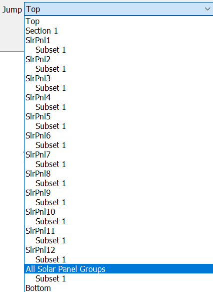
- When the Solar Panel Area report displays, scroll down to the All Solar Panel Group panel.
- Review the report
- Close the Solar Panel Area report.
You can also select All Solar Panel Groups from the Jump To drop-down list.
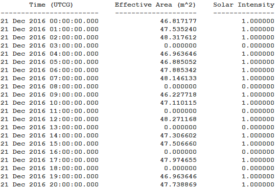
Solar Panel Area Report
The values reported as the Effective Area represent the solar panel area lit by the Sun and reduced by the cosine loss. This area can be readily incorporated in power computations.
Creating a Solar Panel Power graph
Your analysis period starts on the date of the winter solstice in 2016 and lasts until the winter solstice in 2017. Due to the Earth's elliptical orbit, the Earth is at perihelion approximately two weeks after the winter solstice, and at aphelion approximately weeks after the summer solstice.
| Solstice | Date | Time (UTCG) |
|---|---|---|
| Winter Solstice 2016 | 21 Dec 2016 | 10:44 |
| Spring Equinox 2017 | 20 March 2017 | 10:28 |
| Summer Solstice 2017 | 21 June 2017 | 04:24 |
| Fall Equinox 2017 | 22 Sept 2017 | 20:02 |
| Winter Solstice 2017 | 21 Dec 2017 | 16:28 |
The solar panels' effective area changes during the solstice time, and so too does the power. Remember that the solar panels' power generation is directly related to their effective area. You can visualize the changes in power using a Solar Panel Power graph, which is a plot of the power generated by the solar panels illuminated by the Sun over time, captured at each time step.
Generating a new graph
Select the graph option and generate a Solar Panel Power graph.
- Bring the Solar Panel tool to the front.
- Return to the Data Reporting panel.
- Select Power for the Type.
- Select the Graph option.
- Click .
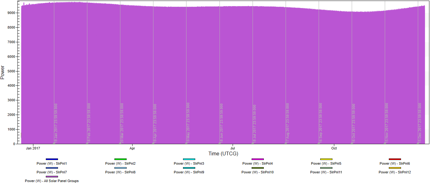
Power graph
Customizing the graph
Update the range of the Y axis by
- Double-click on the graph.
- Select the Axis tab when the Customization dialog box opens.
- Select the Min option in the Y Axis panel.
- Enter 8500 in the Min field.
- Click to confirm you changes and to close the Customization dialog box.
- Review the updated graph.
This is the value in watts.
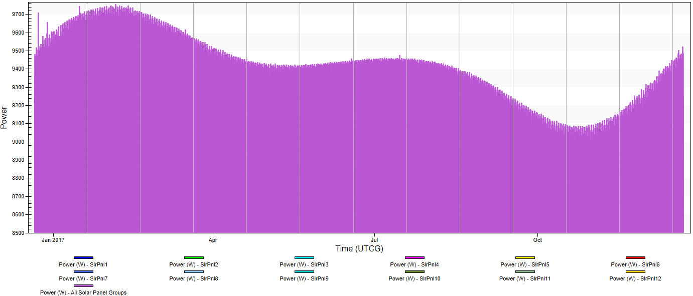
Customized Power graph
Over the course of the year, you can see the measured solar power vary, with the most power being generated around the time of Earth's perihelion and the least around aphelion. The Earth's elliptical orbit and the satellite’s position in orbit and attitude affected the total power generated.
Saving your work
Clean up and close out your scenario.
- Close the Solar Panel Power graph.
- Click to Close the Solar Panel tool.
- Close the Solar Panel View window.
- Save () your work.
- Close the scenario ().
Summary
You created a new scenario to analyze the solar power generation on the NASA Aqua satellite between the winter solstices of 2016 and 2017. After inserting the satellite from the Standard Object Database, you loaded and examined a custom model file, which contained a definition of Aqua's solar panels. You used the Solar Panel tool to compute the solar illumination of the panels over the course of a solar cycle, then reported on the data using a report and graph. By using the Solar Panel tool, you were able to calculate and view the differences in estimated solar panel power generation over time.
On your own
You can view further details about the Aqua satellite's power generation at the time of this scenario here.