STK Pro, STK Premium (Air), STK Premium (Space), or STK Enterprise
You can obtain the necessary licenses for this tutorial by contacting AGI Support at support@agi.com or 1-800-924-7244.
This lesson requires STK 12.9 or newer to complete it in its entirety. If you have an earlier version of STK, you can view a legacy version of this lesson.
The results of the tutorial may vary depending on the user settings and data enabled (online operations, terrain server, dynamic Earth data, etc.). It is acceptable to have different results.
Capabilities covered
This lesson covers the following STK Capabilities:
- STK Pro
- Communications
- Urban Propagation Extension (UProp)
Problem statement
Engineers and operators need to compute diffraction losses in an urban environment and apply them to a link budget. Luckily, urban propagation determines the impact of buildings, terrain, and ground reflections on your communications. They want to assess the effects of urban propagation to plan for link outages and asset redundancy. They are interested in how hand-held communication devices will be affected by buildings and structures. They need to analyze communications from a central location in a city to determine carrier-to-noise ratio throughout the city.
Solution
Use a combination of STK Pro, the Communications and Coverage capabilities, and the Urban Propagation Extension (UProp)’s Urban Propagation Wireless InSite model to create communications coverage in an urban test zone looking for dead zones throughout the city.
What you will learn
Upon completion of this tutorial, you will understand the following:
- How to use the Urban Propagation Extension for STK Communications.
- How to display C/N contours in the 3D Graphics window.
Video guidance
Watch the following video. Then follow the steps below, which incorporate the systems and missions you work on (sample inputs provided).
Using the starter scenario (*.vdf file)
To speed things up and enable you to focus on this lesson's main goal, you will use a partially created scenario. The partially created scenario is saved as a visual data file (VDF) in your STK install.
Retrieving the starter scenario
- Launch the STK (
 ) application.
 - Click
 Open a Scenario in the Welcome to STK dialog box.
 - Go to <Install Dir>\Data\Resources\stktraining\VDFs.
- Select STK_Communications.vdf.
- Click .
Visual data files versus Scenario files
You must make sure that you save your work in the STK application as a scenario file (.sc) and not a visual data file (.vdf) by selecting Save As from the STK File menu. A VDF is a compressed version of an STK scenario, which makes them great for sending your work in the STK application to others. However, you should use a scenario file while working with the STK application on your machine.
If you open a VDF file, the STK application keeps it as a VDF and does not automatically convert it to a scenario file. This means that the STK application does not change the file type of your scenario when you launch your scenario. You need to convert the VDF to a Scenario file using Save As.
Saving a VDF file as a Scenario file
Use Save As from the STK File menu to convert the VDF file that you opened into a scenario file.
- Select Save As... in the File menu.
- Select the STK User folder in the navigation pane.
- Right-click in the file and folder browser.
- Select New > Folder in the shortcut menu.
- Rename New Folder to match the title of the scenario.
- Open the folder you just created.
- Enter the name of the folder into the File name field. This will be the Scenario object's name.
- Open the Save as type drop-down menu.
- Select Scenario Files (*.sc).
- Click .
Analyzing urban communications
In this scenario, you will analyze communications between a central location in a city and grid throughout the city.
Selecting the relevant objects
You will only use a portion of the available objects in the Object Browser in this tutorial, not all of them. There are extra objects because you can use this same scenario to complete other lessons about the STK Communications capability.
- Select the check box for the following objects in the Object Browser:
- Skopje_Extents (
 )
) - Skopje_CommSite (
 )
) - Click Save (
 ).
).
Save (![]() ) often during this lesson!
) often during this lesson!
Changing the analysis period
Since you are analyzing a grid with no moving objects, you can narrow your analysis period to 1 second. This is a trick you can do in STK to shorten your computation time.
- Right-click on your Scenario object (
 ) in the Object Browser.
 - Select Properties (
 ) in the shortcut menu.
 - Select the Basic - Time page when the Properties Browser opens.
- Enter the following in the Analysis Period panel:
- Click to accept your change and to keep the Properties Browser open.
| Option | Value |
|---|---|
| Start | 1 Aug 2022 06:00:00.000 UTCG |
| Stop | + 1 sec |
Using analytical terrain
Use a local terrain file for analysis and visualization.
- Select the Basic - Terrain page. You can see that Use terrain server for analysis is turned off.
- Select the Use check box for SRTM_Skopje.pdtt in the Custom Analysis Terrain Sources panel.
- Click to accept your changes and to keep the Properties Browser open.
Modeling the RF Environment with the Urban Propagation Wireless InSite model
The Urban Propagation Wireless InSite model offers a selection of a deterministic model and four empirical models for calculating path loss between two locations in an urban environment. The deterministic model, Triple Path Geodesic (TPGEODESIC), was developed by Remcom as a derivative of their Wireless InSite 3D propagation loss module, Wireless InSite.
The TPGEODESIC model is a rapid urban propagation model that uses the buildings' 3D geometry data to define an urban environment. The 3D geometry data is used to compute wedge diffractions. The TPGEODESIC model produces higher-fidelity results than empirical models but at greatly reduced computation times compared to full physics-based models.
Enabling the Urban Propagation Wireless InSite model
Use Urban Propagation Wireless InSite to model the RF environment for your link analysis.
- Select the RF - Environment page.
- Select the Urban & Terrestrial tab.
- Select the Use check box.
- Click the Urban Terrestrial Propagation Loss Model Component Selector (
 ).
). - Select Urban Propagation Wireless InSite 64 (
 ) in the Urban Terrestrial Propagation Loss Models list, once the Select Component dialog box opens.
 - Click to close the Select Component dialog box.
- Ensure TPGEODESIC is set for Calculation Method.
Describing the TPGEODESIC calculation method
The deterministic model, which is the default, is the preferred model. It produces higher-fidelity results than empirical models. TPGEODESIC returns the no data value unless it meets this restriction: transmitter and receiver must be outside of buildings and above ground. The TPGEODESIC model provides good general coverage of cityscapes between any pair of antennas not located underground or indoors.
Using an Urban Geometry Data file
The shapefiles for the STK Urban Propagation Extension must have polygon features to represent building footprints and an elevation attribute to represent elevations of the buildings. You should limit the shapefile to a maximum range of three square kilometers. The shapefile may contain holes in its building polygons (e.g., courtyards, shafts, and plazas) but those holes are not recognized either analytically or graphically by the Urban Propagation Extension.
- Click the File ellipsis () in the Urban Geometry Data panel.
- Browse to the Urban building Geometry Data File (typically: <STK install folder>\Data\Resources\stktraining\samples) in the Select File dialog box.
- Select Skopje.shp.
- Click .
Determining the building height data attribute
You can use the data attribute in the Urban Geometry Data file to provide the building height. The Building Height Data Attribute list contains all the columns in the data file. In the Skopje.shp file, the ZV2 column contains the height attribute. When you use HeightAboveTerrain, the calculation determines a building height relative to terrain.
- Open the Data Attribute drop-down list in the Building Height panel.
- Select ZV2.
- Open the Reference Method drop-down list.
- Select Height Above Terrain.
Enabling Terrain Data
You loaded analytical terrain into your scenario. Select this check box to incorporate the effect of terrain in your urban propagation analysis.
- Select the Use Terrain Data check box.
- Click to accept your changes and to close the Properties Browser.
- Click Reset (
 ) in the Animation toolbar.
Visualizing the terrain in the 3D Graphics window
Display the SRTM_Skopje.pdtt and the Skopje shapefile in the 3D Graphics window by zooming to Skopje_Extents (![]() ).
).
- Select the SRTM_Skopje.pdtt check box in Globe Manager.
- Bring the 3D Graphics window to the front.
- Right-click Skopje_Extents () in the Object Browser.
- Select Zoom To in the shortcut menu.
- Use your mouse to zoom in and view the Skopje shapefile and surrounding terrain.
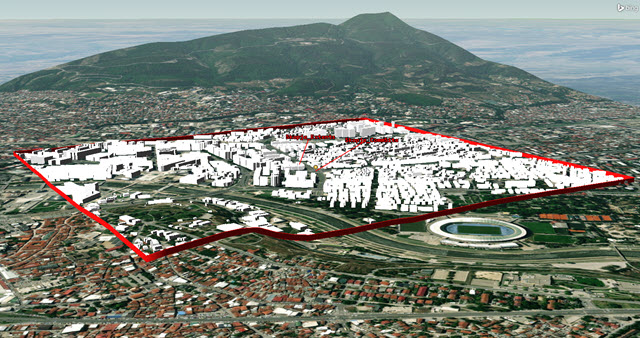
SKOPJE SHAPEFILE
Placing the transmitter in the center of Skopje
The communications site is located approximately in the center of the Skopje shapefile. You can place both the transmitter and receiver at that location.
Inserting a Transmitter object to the Skopje communications site
Add a Transmitter to the Skopje communications site.
- Zoom to Skopje_CommSite ().
- Select Transmitter (
 ) in the Insert STK Objects Tool.
 - Select the Insert Default () method.
- Click .
- Select Skopje_CommSite () in the Select Object dialog box.
- Click .
- Right-click Transmitter1 () in the Object Browser.
- Select Rename.
- Rename Transmitter1 () to TwoWay_Tx.
Using a Complex Transmitter model
Use a Complex Transmitter model for your analysis. When using the Urban Propagation Wireless InSite model, your frequency cannot go below 100 MHz. There is no upper limit restriction; however, above 7 GHz, predictions can become more sensitive to the finer-resolution building details that may not be present in the shapefile or in the model's internal, simplified geometry.
- Open TwoWay_Tx's () Properties ().
- Select the Basic - Definition page.
- Click the Transmitter Model Component Selector ().
- Select Complex Transmitter Model () in the Transmitter Models list.
- Click to accept your selection and to close the Select Component dialog box.
- Select the Model Specs tab.
- Enter the following specifications:
- Click to accept your changes and to keep the Properties Browser open.
| Option | Value |
|---|---|
| Frequency | 450 MHz |
| Power | 4 W |
| Data Rate | 10 Mb/sec |
Using a dipole antenna for the transmitter
Your transmitter uses a dipole antenna.
- Select the Antenna tab.
- Select the Model Specs subtab.
- Click the Antenna Model Component Selector ().
- Select Dipole () in the Antenna Models list.
- Click to accept your change and to close the Select Component dialog box.
- Enter the following specifications:
- Click to accept your changes and to keep the Properties Browser open.
| Option | Value |
|---|---|
| Design Frequency | 450 MHz |
| Length | 0.32 m |
| Efficiency | 80 % |
Adjusting the antenna height
For your analysis, place the antenna six feet above the terrain. Provided that both transmitter and receiver are above ground, there is no height restriction. However, prediction fidelity declines if both the transmitter and receiver are on or close to the ground (less than one meter). This is because ground conditions that are important to the analysis (e.g., ground cancellation) are not included.
- Select the Orientation subtab.
- Enter -6 ft in the Z field in the Position Offset panel.
- Click to accept your changes and to keep the Properties Browser open.
Disabling the line-of-sight and Az-El Mask constraints
You should not employ STK Line of Sight and Az-El Mask constraints. The Triple Path Geodesic model of the Urban Propagation Extension uses a higher-fidelity algorithm to simulate RF propagation in an urban environment than a simple line-of-sight prediction. In particular, the model has the capability to make signal attenuation predictions in situations with an obscured line-of-sight transmission. It does so by considering three of the most significant paths of diffracted energy around buildings and over terrain. Thus, the use of Line of Sight and Az-El/terrain mask constraints is not appropriate when using the Triple Path Geodesic model.
- Select the Constraints - Active page.
- Clear the Enable check box for the Line Of Sight constraint in the Active Constraints list.
- Click to accept your changes and to close the Properties Browser.
Adding a Receiver object to the Skopje communications site
Now you can model the Receiver at the communications site in Skopje.
Inserting a Receiver object
Attach a Receiver (![]() ) object to Skopje_CommSite.
) object to Skopje_CommSite.
- Insert a Receiver (
 ) object using the Insert Default () method.
 - Select Skopje_CommSite () in the Select Object dialog box.
- Click to close the Select Object dialog box.
- Rename Receiver1 () to TwoWay_Rx.
Using a Complex Receiver model
Use a Complex Receiver model for your analysis.
- Open TwoWay_Rx's () Properties ().
- Select the Basic - Definition page.
- Click the Receiver Model Component Selector ().
- Select Complex Receiver Model () in the Receiver Models list.
- Click to accept your selection and to close the Select Component dialog box.
Using a dipole antenna for the receiver
Your receiver uses a dipole antenna.
- Select the Antenna tab.
- Select the Model Specs subtab.
- Click the Antenna Model Component Selector ().
- Select Dipole () in the Antenna Models list.
- Click to accept your change and to close the Select Component dialog box.
- Enter the following specifications:
- Click to accept your changes and to keep the Properties Browser open.
| Option | Value |
|---|---|
| Design Frequency | 450 MHz |
| Length | 0.32 m |
| Efficiency | 80 % |
Adjusting the antenna height
Place the antenna six feet above the terrain.
- Select the Orientation subtab.
- Enter -6 ft in the Z field in the Position Offset panel.
- Click to accept your changes and to keep the Properties Browser open.
Disabling the line-of-sight constraint
Turn off the line-of-sight constraint.
- Select the Constraints - Active page.
- Clear the Enable check box for the Line Of Sight constraint in the Active Constraints list.
- Click to accept your changes and to close the Properties Browser.
Analyze the transmitter broadcast with a Coverage Definition
Determine how well your transmitter can broadcast within the extents of the Skopje shapefile. You can do this by restricting your coverage grid to the Skopje_Extents Area Target object.
Inserting the Coverage Definition object
Use a Coverage Definition (![]() ) object to restrict your coverage grid to the Skopje_Extents Area Target object.
) object to restrict your coverage grid to the Skopje_Extents Area Target object.
- Insert a Coverage Definition (
 ) object using the Insert Default () method.
 - Open CoverageDefinition1's () Properties ().
- Select the Basic - Grid page when the Properties Browser opens.
Adjusting the grid area of interest
Place your coverage grid inside Skopje_Extents (![]() ).
).
- Open the Type drop-down list in the Grid Area of Interest panel.
- Select Custom Regions.
- Select Area Targets in the drop-down list below Custom Regions.
- Move (
 ) Skopje_Extents () from the Area Targets list to the Selected Regions list.
Defining your grid
You are confining your grid to a small geographical area. Therefore, use Distance for the grid spacing.
- Select Distance from the drop-down list in the Point Granularity panel.
- Enter 100 ft in the Distance field.
Adding a grid constraint
Use TwoWay_Rx (![]() ) as the grid constraint.
) as the grid constraint.
- Click .
- Open the Reference Constraint Class drop-down list in the Grid Constraint Options dialog box.
- Select Receiver.
- Select Skopje_CommSite/TwoWay_Rx in the Use Object Instance list.
- Click to close the Grid Constraints Options dialog box.
Adjusting the grid point altitude
You are analyzing communications from your transmitter to your receiver which is constrained to each grid point inside Skopje_Extents (![]() ). Place your grid points at an altitude of six feet above the terrain.
). Place your grid points at an altitude of six feet above the terrain.
- Open the Point Altitude drop-down list.
- Select Altitude above Terrain.
- Enter 6 ft in the Altitude above Terrain field.
- Click to accept your changes and to keep the Properties Browser open.
Selecting assets
Select TwoWay_Tx (![]() ) as your asset.
) as your asset.
- Select the Basic - Assets page.
- Expand (
 ) Skopje_CommSite () in the Assets list.
 - Select TwoWay_Tx ().
- Click .
- Click to accept your changes and to keep the Properties Browser open.
Setting the 3D Graphics fill options
Tell STK to display the Figure Of Merit at altitude in the 3D Graphics window.
- Select the 3D Graphics - Attributes page.
- Select the Show at Altitude check box in the Fill Options panel.
- Click to accept your changes and to close the Properties Browser.
Computing accesses using your Coverage Definition object
The Compute Accesses tool enables you to compute accesses between the grid points and the assigned assets.
- Select CoverageDefinition1 () in the Object Browser.
- Open the CoverageDefinition menu.
- Select Compute Accesses.
Using a Figure of Merit to visualize Coverage
The Coverage Figure of Merit (![]() ) object enables you to analyze coverage in various directions over time, using several attitude-dependent figures of merit.
) object enables you to analyze coverage in various directions over time, using several attitude-dependent figures of merit.
Inserting a Figure of Merit object
Add a Figure of Merit to the Coverage Definition.
- Insert a Figure Of Merit (
 ) object using the Insert Default () method.
 - Select CoverageDefinition1 () in the Select Object dialog box.
- Click to close the Select Object dialog box.
Determining Access Constraints
You are interested in analyzing carrier-to-noise ratio (C/N). Access Constraints is perfect for this analysis. Access Constraints measures the value of various constraint parameters used to define visibility within STK.
- Open FigureOfMerit1's () Properties ().
- Select the Basic - Definition page.
- Set the Definition - Type to Access Constraint.
- Set the following definitions:
- Click to accept your changes and to keep the Properties Browser open.
| Option | Value |
|---|---|
| Constraints | C/N |
| Compute | Maximum |
| Time Step | 1 sec |
Generating Grid Stats report
The Grid Stats report provides minimum, maximum, and average values.
- Right-click FigureOfMerit1 () in the Object Browser.
- Select Report & Graph Manager (
 ) in the shortcut menu.
 - Select Grid Stats (
 ) in the Installed Styles list, once the Report & Graph Manager opens.
 - Click .
- Scroll to the bottom of the Grid Stats report.
- Look at the Maximum (dB) value in the report (e.g., approximately 87 dB). Use this value to create contours in your 2D and 3D Graphics windows.
- Close the Grid Stats report and the Report & Graph Manager.
Defining static graphics for the Figure of Merit
The Static page enables you to define static graphics for a Figure Of Merit object.
- Return to FigureOfMerit1's () Properties ().
- Select the 2D Graphics - Static page.
Adjusting translucency
Have the 2D and 3D Graphics windows display the points as filled polygons and set the translucency.
- Enter 25.00 in the % Translucency field.
Adding levels
You can specify how levels of coverage quality appear in both the 2D and 3D Graphics windows. You are not interested in any areas where the C/N is below five (5) dB, so round down your maximum C/N dB value to 85 dB.
- Select the Show Contours option in the Display Metric panel.
- Set the following Level Adding values:
- Click .
| Option | Value |
|---|---|
| Start | 5 dB |
| Stop | 85 dB |
| Step | 5 dB |
Adjusting the levels' attributes
Using the Color Ramp enables you to apply a spectrum pattern with selected start and end colors.
- Ensure the Color Method is set to Color Ramp.
- Open the Start Color drop-down list.
- Select red.
- Open the End Color drop-down list.
- Select blue.
Using Natural Neighbor contour interpolation
Use Natural Neighbor, which applies color smoothly over all points in the grid to differentiate contour levels.
- Select the Natural Neighbor option in the Contour Interpolation (points must be filled) panel.
- Click to accept your changes and to keep the Properties Browser open.
Displaying contour legends
The Legend provides you with a convenient way to interpret contour data displayed in the 2D and 3D Graphics windows.
- Click in the Levels panel.
- Click when the Static Legend for FigureOfMerit1 opens.
- Select the Show at Pixel Location check box in the 2D Graphics Window panel.
- Select the Show at Pixel Location check box in the 3D Graphics Window panel.
- Type Carrier to Noise Ratio (dB) in the Title field in the Text Options panel.
- Enter 0 in the Number Of Decimal Digits field.
- Enter 50 in the Color Square Width (pixels) field in the Range Color options panel.
- Click to close the Figure of Merit Legend Layout dialog box.
- Close (
 ) the Static Legend for FigureOfMerit1.
 - Click to close FigureOfMerit1's () Properties ().
Viewing the contours in the 3D Graphics window
You can view the contours in both the 2D and 3D Graphics windows. Use the 3D Graphics window.
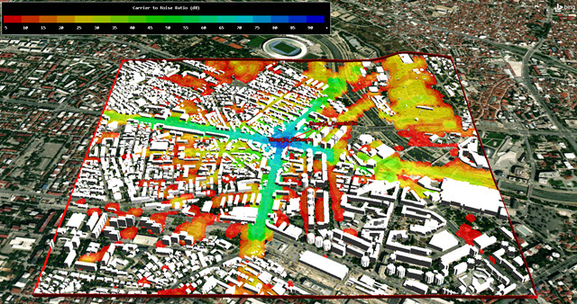
C/N CONTOURS
The view is a great way to brief anyone located at the city intersection on where anyone else with a hand-held receiver can expect to have communications with you. Areas on the map with no color are below the 5 dB C/N cutoff.
Summary
This tutorial introduced you to Urban Propagation Wireless InSite Model capabilities using wide-area coverage. You used a meticulously built shapefile to simulate structures inside an urban environment. Using RF Environment, you loaded the shapefile analytically using the Urban Propagation Wireless InSite model. You placed a Complex Transmitter and Receiver model at a central location in the city. Next, you built a Coverage Definition object and confined the coverage grid to the shapefile's extents. You placed the receiver's constraints at each grid point and selected the transmitter as the asset. You set your figure of merit to access constraint, focusing on carrier-to-noise ratio, and determined where your ratios would fall below five (5) dB using color contours inside your graphics window.
Saving your work
Clean up your workspace and save your scenario.
- Close any open reports, properties and tools.
- Save () your work.
On your own
Find specifications for a drone hand-held transmitter and update the Transmitter object's properties while keeping the transmitter in the same central location. Raise the receiver to 400 feet in the Coverage Definition setup, which is the typical allowed maximum altitude for recreational pilots. Compute coverage at that altitude. You could create a flight route using an Aircraft object and perform single object coverage at altitude or simply create a link budget. You can move the transmitter to a different location, raise its antenna height and keep the receiver at six (6) feet and perform coverage. There are many variations that you can apply to make this STK capability so interesting.