STK Premium (Air) and STK Premium (Space) or STK Enterprise
You can obtain the necessary licenses for this tutorial by contacting AGI Support at support@agi.com or 1-800-924-7244.
The results of the tutorial may vary depending on the user settings and data enabled (online operations, terrain server, dynamic Earth data, etc.). It is acceptable to have different results.
Capabilities covered
This lesson covers the following capabilities of the Ansys Systems Tool Kit® (STK®) digital mission engineering software:
- STK Pro
- STK SatPro
- Aviator
- Communications
- Analysis Workbench
- Coverage
- Volumetric Analysis
Problem statement
Engineers and analysts require an efficient way to create constellations of satellites with similar payloads. They may also need to determine if receivers on those satellites will sustain interference from other communication devices. You want to evaluate an aircraft's communications link with a constellation of satellites in low Earth orbit (LEO) as the aircraft flies a search pattern. The testbed aircraft is outfitted with a phased array communication antenna. You need to evaluate the additional RF energy which may interfere with other satellites in LEO, medium Earth orbit (MEO), and geostationary Earth orbit (GEO).
Solution
Use the STK software and the SatPro capability's Walker Tool to create a constellation of satellites. Next, create an Aircraft object that flies a search pattern in a designated area of interest using the STK software's Aviator capability. You will use a CommSystem object, part of the Communications capability, to determine possible communication interference with the LEO satellites and evaluate the carrier-to-noise ratio (C/N). Finally, you will use the Analysis Workbench and Volumetric Analysis capabilities to visualize potential radio frequency interference in the LEO, MEO and GEO volume of space.
What you will learn
Upon completion of this lesson, you will understand the following:
- The Walker Tool
- Aviator Area Target Search patterns
- The CommSystem object
- The Spatial Analysis tool
- The Volumetric object
Creating a new scenario
You will create a new scenario with a run time of five hours.
- Launch the STK application (
 ).
). - Click Create a Scenario (
 ) in the Welcome to STK dialog box.
 - Enter the following in the STK: New Scenario Wizard:
- Click when you finish.
- Click Save (
 ) once the scenario loads. A folder with the same name as your scenario is created for you.
 - Verify the scenario name and location.
- Click .
| Option | Value |
|---|---|
| Name | Volumetrics_CN |
| Start | 15 Mar 2022 16:00:00.000 UTCG |
| Stop | + 5 hrs |
Save (![]() ) often!
) often!
Creating a LEO constellation
You will use a Walker constellation to model the constellation of LEO satellites. Each satellite will have a hemispherical nadir pointing antenna. In order to define the walker constellation, you first need to create a "seed" satellite to define the general orbital parameters.
Understanding Walker constellations
The Walker Tool, available as part of the STK Software's
The way in which spacing between the ascending nodes that define the orbital planes is calculated depends on the type of Walker constellation you choose. In addition to specifying the number of satellites in each plane, you must also specify the location of the first satellite in each plane relative to the first satellite in adjacent planes. The way to specify the position of the first satellite depends on the type of Walker constellation you choose.
| Type | Description |
|---|---|
| Delta | Delta configurations have orbit planes distributed evenly over a span of 360 degrees in right ascension. Requires an integer value of f for inter-plane phasing. |
| Star | Star configurations have orbit planes distributed over a span of 180 degrees. Requires an integer value of f for inter-plane phasing. |
| Custom | A Custom configuration allows for explicit input of the span over which ascending nodes should be distributed and allows for the explicit specification of inter-plane phasing in terms of a true anomaly offset. |
Creating a seed satellite
First, define a satellite with the characteristics and orbit you need, then, use the Walker Tool to create a Walker constellation. The original satellite that is used to create the Walker constellation is referred to as the "seed" satellite, while the satellites generated using the Walker Tool are referred to as Child satellites. Use the Orbit Wizard to create the "seed" satellite from which the other satellites will be derived.
- Select Satellite (
 ) in the Insert STK Objects tool (
 ).
). - Select the Orbit Wizard (
 ) method.
 - Click .
- Set the following options in the Orbit Wizard:
- Click to confirm your selections and to insert the seed satellite.
| Option | Value |
|---|---|
| Type | Repeating Ground Trace |
| Satellite | LEO_Sat |
| Approximate Altitude | 800 km |
| Color | White |
Modeling the LEO satellite's receiver
Insert a Receiver object which will function as the receiver on the LEO satellite and all of its children. You will use a Complex Receiver model. A Complex Receiver Model enables you to select among a variety of analytical and realistic antenna models and to define the characteristics of the selected antenna type.
- Insert a Receiver (
 ) object using the Define Properties (
 ) method.
 - Select LEO_Sat () in the Select Object dialog box.
- Click .
- Select the Basic - Definition page.
- Click the Receiver Model Component Selector (
 ).
). - Select Complex Receiver Model (
 ) in the Select Component dialog box.
 - Click to confirm your selection and to close the Select Component dialog box.
Selecting the Receiver's antenna model
Use the Basic Definition page for a receiver, transmitter, radar, or antenna object to select an antenna model type from the Component Browser.
- Select the Antenna tab.
- Click the Antenna Models Component Selector ().
- Select Hemispherical ().
- Click to confirm your selection and to close the Select Component dialog box.
- Click to save your changes and to keep the Properties Browser open.
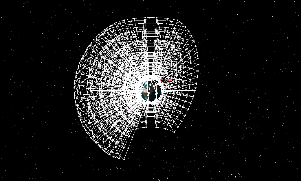
A Hemispherical antenna type provides a built-in model antenna gain pattern covering half of the hemisphere along the boresight.
Visualizing the antenna pattern
Display the shape and volume of the antenna pattern using the receiver's 3D Graphics – Attributes page.
- Select the 3D Graphics – Attributes page.
- Select the Show Volume check box.
- Click .
- Right-click on Receiver1 () in the Object Browser.
- Select Rename the shortcut menu.
- Rename Receiver1 () LEO_Rx.
- Right-click on LEO_Sat () in the Object Browser.
- Select Zoom To in the shortcut menu.
- Bring the 3D Graphics window to the front.
- Use your mouse to get a good view of the satellite and the antenna pattern.

Hemispherical Antenna Pattern
Creating a Walker constellation
Using the seed satellite, create a constellation with orbital characteristics that provide global coverage. You will design a constellation that has at least one satellite in view of the aircraft at all times.
- Right-click on LEO_Sat () in the Object Browser.
- Select Satellite in the shortcut menu.
- Select Walker... in the Satellite submenu.
- Enter the following in the Walker Tool:
- Click to insert the Walker constellation.
- Click to close the Walker Tool.
| Option | Value |
|---|---|
| Type | Delta |
| Number of Sats per Plane | 10 |
| Number of Planes | 10 |
| Color by Plane | Cleared |
If the seed satellite contains child objects such as Receiver objects, the sub-objects are also created for each of the child satellites.
Clearing the seed satellite
When a Walker constellation is created, each child has the same base name as the seed satellite plus two numbers. The first number identifies the plane in which the satellite resides and the second identifies the satellite's position in the plane. In this case, you've created a Walker constellation with two planes and ten satellites per plane, LEO_Sat0102 is the second satellite in the first plane. If you keep the seed satellite in the scenario, two identically configured satellites (the seed satellite and the first satellite in the first plane) will be considered in your analysis. To prevent duplicate analysis, remove the seed satellite.
- Save () your scenario.
- Select LEO_Sat () in the Object Browser.
- Click Delete (
 ).
). - Click to confirm your deletion when the Delete Object dialog box opens.
When you save the scenario, all objects in the scenario are also saved. It is important that you save the scenario before you remove LEO_Sat in case you need to reload it later for further analysis.
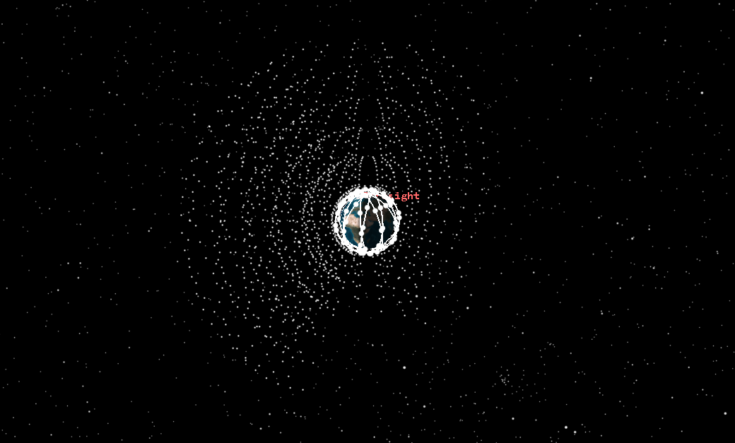
Viewing the LEO satellite constellation
View your Walker constellation in the 3D Graphics window.
- Bring the 3D Graphics window to the front.
- Click Home View (
 ) in the 3D Graphics window toolbar.
 - Use your mouse to turn the Earth in order to view the constellation of LEO satellites.
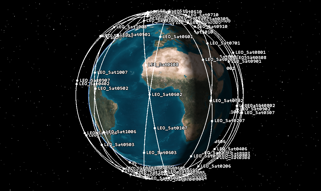
LEO Constellation
Creating the test area
Use an
- Insert an Area Target (
 ) object using the Define Properties () method.
 - Select the Basic - Boundary page
- Click four times in the Points panel to add four points to the Points table.
- Set the following values for the perimeter points in the order shown:
- Click .
- Select the 2D Graphics - Attributes page.
- Clear the Inherit from Scenario check box in the Inheritable Settings panel.
- Clear the Show Label and Show Centroid check boxes.
- Click .
- Rename AreaTarget1 () Test_Area.
The Points table displays a summary of the latitude and longitude values for each perimeter point.
| Latitude | Longitude |
|---|---|
| 34 deg | -121 deg |
| 34 deg | -119 deg |
| 32 deg | -119 deg |
| 32 deg | -121 deg |
Creating the test aircraft
Create and define your aircraft, which is serving as a communications testbed. It is equipped with a phased array antenna and will fly a search pattern inside of a designated test area.
Inserting a new Aircraft object
Use Aviator to propagate the aircraft. With Aviator, the aircraft's route is modeled by a sequence of curves parameterized by well-known performance characteristics of aircraft, including cruise airspeed, climb rate, roll rate, and bank angle.
- Insert an Aircraft object (
 ) using the Insert Default () method.
 - Click .
- Open Aircraft1's () Properties ().
- Ensure the Basic - Route page is selected
- Select Aviator in the Propagator drop-down list.
Selecting the aircraft model
You are using a twin-engine turboprop aircraft for the test. Select a predefined
- Click Select Aircraft (
 ) in the Initial Aircraft Setup toolbar.
 - Select Basic Turboprop (
 ) in the User Aircraft Models (
 ) list when the Select Aircraft dialog box opens.
 - Click to confirm your selection and to close the Select Aircraft dialog box.
- Click .
- Rename Aircraft1 () TestAircraft.
Inserting an Area Target site
You can use an Area Target as a site for an Aviator procedure. The site defines the location (excluding altitude) of the procedure and the types of procedures that are available to select. The exact relationship between the site location and the procedure is dependent on the specific procedure.
- Right-click on Phase 1 (
 ) in the Mission List.
 - Select Insert First Procedure for Phase ... (
 ) in the shortcut menu.
 - Select STK Area Target (
 ) in the Select Site Type list.
 - Click .
Configuring an Area Target Search procedure
An
- Select AreaTargetSearch () in the Select Procedure Type list.
- Clear the Use Aircraft Default Cruise Altitude check box in the Altidude panel.
- Enter 10000 ft in the Altitude field.
- Set the following options in the Search Options panel:
- Change Turn Factor to 2 in the Enroute Options panel.
- Ensure Max Range Airspeed is selected in the Enroute Cruise Airspeed panel.
- Click .
- Click .
- Click when the Flight Path Warning window appears.
- Click .
| Option | Value |
|---|---|
| Max Separation | 10 nm |
| Course Mode | Override |
| Centroid True Course | 180 deg |
The search pattern is based on the course defined for the area target's centroid. The STK software's Aviator capability will fill the search area with parallel flight lines derived from the centroid's course, and the point of entry to the search pattern is defined relative to that course.
This is a variable airspeed that maximizes the distance the aircraft can fly.
Viewing the search pattern in the 3D Graphics window
Review your changes in the 3D Graphics window.
- Bring the 3D Graphics window to the front.
- Right-click on Test_Area () in the Object Browser.
- Select Zoom To in the shortcut menu.
- Click Orient North (
 ).
). - Zoom out until you can see the full extent of the test area and the aircraft's flight route.
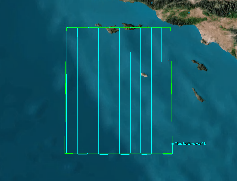
Aircraft Search Pattern
Building the aircraft's transmitter
Define the transmitter you are using for the tests. You will use a
- Insert a Transmitter (
 ) object using the Define Properties () method.
 - Select TestAircraft () in the Select Object dialog box.
- Click .
- Select the Basic - Definition page.
- Select the Transmitter Model Component Selector ().
- Select the Complex Transmitter Model () in the Select Component dialog box.
- Click .
- Select the Model Specs tab.
- Set Power to 40 dBW.
- Click .
Modeling the phased array transmitter antenna
Select a Phased Array antenna model from the Component Browser and define its characteristics. A
- Select the Antenna tab.
- Ensure the Model Specs sub-tab is selected.
- Select the Antenna Model Component Selector ().
- Select Phased Array () in the Select Component dialog box.
- Click .
- Ensure the Element configuration sub-sub tab is selected.
- Enter 9 in the X field in the Number of Elements panel.
- Enter 9 in the Y field in the Number of Elements panel.
The Element Configuration tab enables you to define the physical aspects of the antenna elements.
Updating the beam target
Use the Beam Direction Provider sub-sub-tab to select where the antenna points its beam. By modifying the excitation (amplitude and phase) of each element differently, a phased array antenna can electronically steer its maximum gain toward a particular direction or main radiation axis.
- Select the Beam Direction Provider sub-sub-tab.
- Select the Enabled check box in the Beam Steering panel.
- Click in the Selection Filter panel.
- Select the Satellite () check box in the Selection Filter panel.
- Move (
 ) all of the satellites to the beam target list.
 - Click .
Updating the antenna's orientation
The STK software provides
- Select the Orientation sub-tab.
- Set the Elevation to -90 deg.
- Set Z to -1.9 ft in the Position Offset panel.
- Click .
An antenna on a vehicle has a default alignment in which the antenna boresight looks down the +Z axis of the vehicle. The default vehicle attitude ("Nadir aligned with ECI velocity vector constraint" for satellites, and "Nadir aligned with ECF velocity vector constraint" for other vehicles) results in the antenna boresight pointing straight down toward the center of the Earth, so an elevation of -90 degrees points the antenna boresight straight up, not down.
This will place the antenna on top of the aircraft's fuselage.
Visualizing the antenna pattern
You want to visualize the antenna pattern as a 3D volume.
- Select the 3D Graphics - Attributes page.
- Set the following options in the Volume Graphics panel:
- Select the Set azimuth and elevation resolution together check box in the Pattern panel.
- Click .
| Option | Value |
|---|---|
| Show Volume | Selected |
| Gain Scale (per dB) | 0.0005 km |
| Minimum Displayed Gain | -20 dB |
Displaying the boresight vector
The boresight vector is a unit vector along the Body Z axis. The Vector is fixed by its components in reference axes.
- Select the 3D Graphics - Vector page.
- Select the Show check box for the Boresight Vector option.
- Click .
- Rename Transmitter1 () to TestAircraft_Tx.
- Right-click on TestAircraft () in the Object Browser.
- Select Zoom To in the shortcut menu.
- Bring the 3D Graphics window to the front.
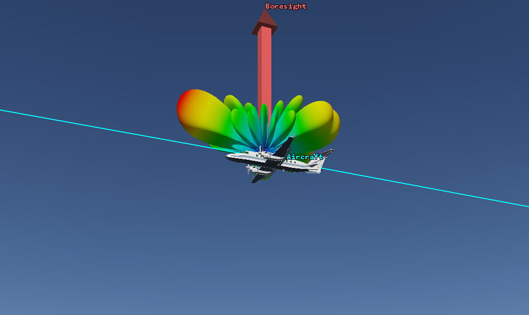
Antenna Pattern and Boresight vector
Plotting C/N along the flight route
There are a couple of ways to approach this problem. Mission planners could use a Chain object and create a link between the test aircraft's transmitter and whatever LEO receivers are in view. Or they could employ a CommSystem object and direct the phased array's main lobe gain towards the LEO satellite that is has the best overhead elevation angle when multiple satellites are in view. Mission planners have decided on the latter.
Organizing the communication system
The STK software's Communications capability provides a CommSystem object that allows you to model dynamically configured communications links between constellations of transmitters and receivers. CommSystems are particularly useful for modeling low and medium Earth orbiting (LEO and MEO) satellite systems. To set up a CommSystem object, you must first organize the relevant communication assets:
- the transmitter(s) in the communications link of interest
- the receiver(s) in the communications link of interest
You can organize the communications assets using
- Insert a Constellation (
 ) object into the scenario using the Insert Default () method.
 - Rename Constellation1 () object Transmitter.
- Insert another Constellation () object into the scenario using the Insert Default () method.
- Rename Constellation2 () object Receivers.
Creating the Transmitter constellation
Add the test aircraft's transmitter to the Transmitter constellation.
- Open Transmitter’s () Properties ().
- Select the Basic - Definition page.
- Select TestAircraft_Tx () in the Available Objects list.
- Move () TestAircraft_Tx () to the Assigned Objects list.
- Click .
Creating the Receivers constellation
Add the satellites' receivers to the Receivers constellation.
- Open Receivers' () Properties ().
- Select the Basic - Definition page.
- Select the Receiver () check box in the Selection Filter list.
- Move () all the receivers to the Assigned Objects list.
- Click .
Building the communications system
- Insert a CommSystem (
 ) object using the Insert Default () method.
 - Open CommSystem1’s () Properties ().
- Select the Basic - Transmit page.
- Select Transmitter () in the Available Constellations list.
- Move () Transmitter () from the Available Constellations list to the Assigned Constellation list.
- Select the Basic - Receive page.
- Select Receivers () in the Available Constellations list.
- Move () Receivers () from the Available Constellations list to the Assigned Constellation list.
If the CommSystem (![]() ) object does not appear in the Insert STK Objects tool, click and select the Show check box to display the object in the Insert STK Objects tool.
) object does not appear in the Insert STK Objects tool, click and select the Show check box to display the object in the Insert STK Objects tool.
Constraining the communications links
Complex communication systems may present many potential links for a given receiver or transmitter. You must
- Select the Basic - Link Definition page.
- Select the Transmit option in the Constraining Constellations panel.
- Leave the Link Selection Criteria set at Minimum Range.
- Click .
Constraining Constellations will generally, but not always, comprise the objects closest to the Earth. Only one link will be established for each object contained within the constraining constellations.
Minimum Range selects the non-constraining objects (the satellite receivers) with the minimum distance to the constraining object (the test aircraft’s transmitter). Basically, you're forcing the phased array antenna to talk to the nearest satellite.
Computing the CommSystem and plotting C/N
After defining your CommSystem, set the CommSystem object to process link information. Because of the dynamic nature of these more complex systems, the CommSystem performs a more traditional analysis by implementing a simulation in which time is advanced over the specified interval at fixed time steps and in which the links are analyzed at each step. The resulting data are available after the simulation is complete for reporting or graphing purposes.
- Right-click on CommSystem1 () in the Object Browser.
- Select CommSystem in the shortcut menu.
- Select Compute Data in the CommSystem submenu.
When you select Compute Data, a two-phase process begins to generate the desired information. The first phase analyzes the visibility of the transmitters, receivers, and interference sources (if available) to each other to determine when they are accessible. Access calculations take into account any of the normal access constraints that may be applied to each of the objects. The second phase steps through the desired CommSystem interval, calculating the link performance. During each of the phases, a Progress window appears. The first phase of calculations is completed rather quickly but the second phase can be lengthy, depending on the complexity of the CommSystem. After link performance and interference are calculated, the desired links, interference sources, and the primary interferer appear in the 2D and 3D Graphics windows.
Be patient! Due to the amount of receivers in the scenario, the computation can take a few minutes.
Generating a Carrier to Noise vs. Time graph
The STK software's Communications capability provides report and graph elements for CommSystems. Use the predefined Carrier to Noise vs Time graph to view C/N over the course of the mission.
- Right-click on CommSystem1 () in the Object Browser.
- Select Report & Graph Manager... (
 ).
). - Select the Carrier to Noise vs Time (
 ) graph in the Installed Styles list.
 - Click .
- Click when the graph opens.
- Change Step to 1 sec.
- Click Refresh (F5) (
 ) in the graph toolbar.
 - Close the graph and the Report and Graph manager when you are finished.
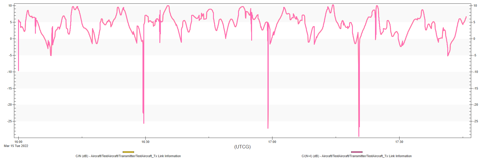
C/N Over Time
You can see that there are several instances where C/N is affected.
Analyzing the RF output throughout MEO with a Volumetric object
You would like to ensure that the RF energy used for your communications link doesn’t interfere with other satellite communications beyond MEO to GEO. In order to evaluate C/N across the MEO, you can define a scalar calculation using the Analysis Workbench capability to a grid template object, and have that grid template object move to all the grid point locations defined in a Volumetric object, which is part of the STK software's Volumetric Analysis capability.
Creating the Volumetric object
A
- Insert a Volumetric (
 ) object using the Insert Default () method.
 - Rename Volumetric1 () to Vol_CN.
Creating a new Volume Grid component
Select a Volume Grid component from Analysis Workbench.
- Open Vol_CN's () Properties ().
- Select the Basic - Definition page.
- Click the Volume Grid ellipsis ().
- Click Create new Volumetric Grid (
 ) when the Select Volume Grid for CN_Vol dialog box opens.
 - Click next to the Type field.
- Select Cartographic in the Select Component Type list when the Select Component Type dialog box opens.
- Click to confirm your selection and to close the Select Component Type dialog box.
- Enter MEO_West in the Name field.
A Cartographic grid uses latitude, longitude and altitude based on the central body reference ellipsoid.
Setting and defining the volume grid values
Add the
- Click .
- Set the following options in the Longitude panel when the Grid Values dialog box opens:
- Set the following options in the Altitude panel:
| Option | Value |
|---|---|
| Minimum | -180 deg |
| Maximum | 0 deg |
| Number of Steps | 10 |
| Option | Value |
|---|---|
| Minimum | 2000 km |
| Maximum | 36000 km |
| Number of Steps | 5 |
- Click to close the Grid Values dialog box.
- Click to close the Add Volumetric Component dialog box.
- Select MEO_West in the Volume Grids for: Earth list.
- Click .
- Click .
Viewing the volume grid
View your changes in the 3D Graphics window.
- Bring the 3D Graphics window to the front
- Click Home View () in the 3D Graphics window toolbar.
- Use your mouse to view the Cartographic Grid (MEO_West).
MEO_West Cartographic Grid
Changing the view
Use the
- Return to Vol_CN's () Properties ().
- Select the 3D Graphics - Grid page.
- Change Size to 2 in the Show grid points field.
- Clear the Show grid lines check box.
- Click .
- Return to the 3D Graphics window to view your changes.
MEO_West Grid Points Only
Defining the volumetric grid
You can use one of the satellites' receivers as the volumetric grid template object. In order to do this, you will need to compute an access from the aircraft transmitter to that receiver so that the scalar calculation for C/N will exist.
- Right-click on TestAircraft_Tx () in the Object Browser.
- Select Access... (
 ) in the shortcut menu.
 - Expand (
 ) LEO_Sat0101 () in the Associated Objects list when the Access Tool opens.
 - Select LEO_Rx1().
- Click
 .
. - Click to close the Access tool.
Using the Spatial Analysis Tool
Use the
You have computed access from the test aircraft’s transmitter to the LEO satellite receiver. The STK software's Analysis Workbench capability has automatically created scalar calculations for all the available communications calculations, including C/N. Next, create a spatial calculation that will move the template object to each point in the volumetric grid and compute C/N at those locations.
- Right-click on LEO_Sat0101 () in the Object Browser.
- Select Analysis Workbench... (
 ) in the shortcut menu.
 - Select the Spatial Analysis tab when Analysis Workbench opens.
Creating a new spatial calculation
A
- Click Create new Spatial Calculation (
 ).
). - Ensure that the Type is set to Scalar At Location.
- Enter CN in the Name field.
- Click the Scalar ellipsis ().
- Select Aircraft-TestAircraft-TransmitterTestAircraft_Tx-To-Satellite-LEO_Sat0101-Receiver-LEO_Rx1 (
 ) in the objects list when the Select Reference Scalar Calculation dialog box opens.
 - Expand () CommLinkInformation (
 ) in the Scalar Calculations for: Aircraft-TestAircraft-Transmitter-TestAircraft_Tx-To-Satellite-LEO_Sat0101-Receiver-LEO_Rx1 list.
 - Select C/N ().
- Click to close the Select Reference Scalar Calculation dialog box.
- Click to close the Add Spatial Analysis Component dialog box.
- Click to close the Analysis Workbench.
This spatial calculation is defined by placing its parent object at various locations on the grid and evaluating the selected (non-spatial) Scalar Calculation from the Calculation tool.
Updating the volumetric object to use the C/N spatial calculation
Now that you have created the C/N spatial calculation, configure the Volumetric object to use that spatial calculation.
- Return to Vol_CN's () Properties ().
- Select the Basic - Definition page.
- Select the Spatial Calculation check box.
- Click the Spatial Calculation ellipsis ().
- Select LEO_Sat0101 () in the object list when the Select Spatial Calculation for Vol_CN dialog box opens.
- Select CN () in the Spatial Calculations for: LEO_Sat0101 list.
- Click to close the Select Spatial Calculation for Vol_CN dialog box.
- Click .
Computing the volumetric analysis
Volumetric Analysis is likely to be more computationally expensive that 2D analysis because extending grids to three dimensions can greatly increase the number of grid points.
- Right-click on Vol_CN () in the Object Browser.
- Select Volumetric in the shortcut menu.
- Click Compute in Parallel in the Volumetric submenu.
Be patient! Due to the amount of receivers and grid points in the scenario, the computation can take a few minutes.
Configuring the volumetric basic interval
To animate the scenario, the Volumetric Analysis capability will need to recompute the data at every time step. In order to compute all of the data beforehand to animate smoothly, adjust the
- Return to Vol_CN's () Properties ().
- Select the Basic - Interval page.
- Select the At times at step size check box in the Evaluation of Spatial Calculation panel.
- Enter 5 min in the At times at step size field.
- Click .
On your own, you can adjust this value to what works for you. Any changes you make will be applied to the spatial calculation limits in the 3D Graphics - Volume page. Therefore, you may want to redo your fill levels.
Be patient. This could take a few minutes.
Configuring volumetric graphics
Spatial Calculation Levels represent straight line distances from the parent object. You can set them on the
- Select the 3D Graphics - Volume page.
- Select the Spatial Calculation Levels option.
- Click .
- Set the following options in the Insert Evenly Spaced Values dialog box:
- Click .
- Click .
When the Spatial Calculation Levels option is selected, the minimum and maximum limits of the spatial calculation can be seen at the top of the page in the Limits panel. Your values may be different.
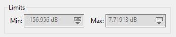
Spatial Calculation Limits
| Option | Value |
|---|---|
| Units | dB |
| Start Value | -10 |
| Stop Value | Round down to the highest Max integer |
| Step Size | 3 |
The start value could be any value you choose; in this instance, it's an arbitrary value. For this scenario you're saying a C/N of -10 dB or higher could create interference.
Setting the 3D Graphics legends
Use the Volumetric
- Select the 3D Graphics – Legends page.
- Select the Show Legend check box.
- Set the following options in the Text Options panel:
- Set the following options in the Range Color Options panel:
- Click .
| Option | Value |
|---|---|
| Title | C/N (dB) |
| Number Of Decimal Digits | 0 |
| Option | Value |
|---|---|
| Max Color Squares per Row | 40 |
| Color Square Width (pixels) | 50 |
Viewing C/N in the 3D volume of space
View your dynamic volumetric object in the 3D Graphics window.
- Bring the 3D Graphics window to the front.
- Reset (
 ) your scenario.
 - Click Normal Animation Mode (
 ) in the Animation toolbar.
 - Decrease Time Step (
 ) to 30 seconds in the Animation Toolbar.
 - Click the Home View ().
- Zoom out so you can see the whole airspace.
- Start (
 ) the animation.
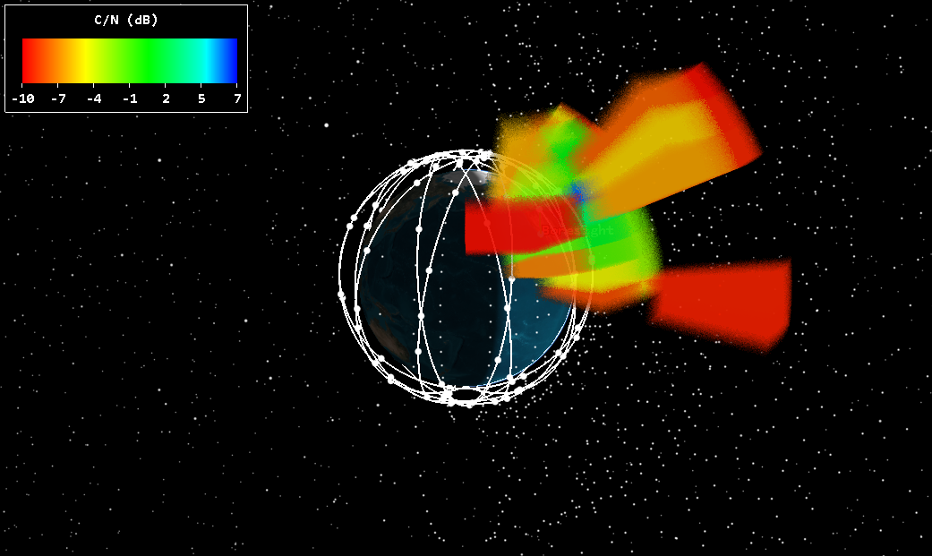
C/N 3D Graphics
You can see that C/N changes every five minutes.
Saving your work
Close out the scenario and save your work.
- Reset () the scenario when you are finished.
- Close any reports or tools that are still open.
- Save () your work.
Summary
You started by creating a constellation of LEO satellites using Walker tool; each satellite had receiver. Next, you designed an Aircraft object that flew a search pattern in a designated area of interest using the Aviator propagator. You utilized the CommSystem object to determine possible communication interference with the LEO satellites. Finally you will created a Volumetric object using the Spatial Analysis tool to create a custom grid to visualize potential radio frequency interference in the LEO, MEO and GEO volume of space.
On your own
Throughout the lesson, hyperlinks were provided that pointed to in depth information. Now's a good time to go back through this tutorial and view that information. Create your own satellite constellation with receivers and a static ground site and transmitter to evaluate interference and apply it to your own custom grid.