STK Pro, STK Premium (Air), STK Premium (Space), or STK Enterprise
You can obtain the necessary licenses for this tutorial by contacting AGI Support at support@agi.com or 1-800-924-7244.
The results of the tutorial may vary depending on the user settings and data enabled (online operations, terrain server, dynamic Earth data, etc.). It is acceptable to have different results.
Capabilities covered
This lesson covers the following capabilities of the Ansys Systems Tool Kit® (STK®) digital mission engineering software:
- STK Pro
- Analysis Workbench
Problem statement
Engineers, analysts, and mission planners need to visualize geometric components with time-varying placement and/or orientation in 3D space for a variety of purposes. You are planning a satellite mission. You want to create both static and dynamic visual aids using vector geometry components of the vehicle's attitude, sensor pointing, and other phenomena of interest. You need a quick and easy way to visualize them clearly and intelligibly.
Solution
Use the Analysis Workbench capability's Vector Geometry tool to configure vector geometry components for the satellite. Then, use the 3D Attitude Graphics window to display an attitude sphere and other pre-built and custom components to create static and dynamic vector graphics for the mission.
What you will learn
Upon completion of this tutorial, you will understand the following:
- How to use the Vector Geometry tool
- How to open and use the 3D Attitude Graphics window
- How to display vector geometry components in 3D Graphics and 3D Attitude Graphics windows
- How to use the attitude sphere as a visualization aid
- How to create a persistent vector display
Creating a new scenario
First, you must create a new scenario, and then build from there.
- Launch the STK application (
 ).
). - Click
 Create a Scenario in the Welcome to STK dialog box.
 - Enter the following in the STK: New Scenario Wizard:
- Click when you finish.
- Click Save (
 ) when the scenario loads.
 - Verify the scenario name and location in the Save As dialog box.
- Click .
| Option | Value |
|---|---|
| Name | AnalysisWorkbench_VGT |
| Location | Default |
| Start | Default |
| Stop | Default |
The STK application creates a folder with the same name as your scenario for you.
Save () often during this scenario!
Disabling streaming terrain
By default, the STK application connects to the Ansys Geospatial Data Cloud to distribute Earth terrain data for analysis and visualization. Turn off
- Right-click on AnalysisWorkbench_VGT () in the Object Browser.
- Select Properties (
 ) in the shortcut menu.
 - Select the Basic - Terrain page when the Properties Browser opens.
- Clear the Use terrain server for analysis check box in the Terrain Server panel.
- Click to confirm your change and to close the Properties Browser.
Modeling a satellite
For this scenario, you will model a notional satellite in a Molniya orbit. Molniya orbits are highly eccentric, meaning that there is a large difference between the altitude at apogee and the altitude of perigee. Molniya orbits are also critically inclined. This keeps the perigee of the orbit in the Southern Hemisphere. Molniya orbits also have a long dwell time in the extreme latitude regions of the Northern Hemisphere.
Inserting a Satellite object
A Satellite object models the properties and behavior of a vehicle in orbit around a central body.
- Bring the Insert STK Objects tool (
 ) to the front.
 - Select Satellite (
 ) in the Select An Object To Be Inserted list.
 - Select the Orbit Wizard (
 ) in the Select A Method list.
 - Click .
Using the Orbit Wizard
The Orbit Wizard is a satellite-level tool designed to assist you in creating any one of several standard orbits or designing your own satellite orbit.
- Open the Type drop-down list when the Orbit Wizard opens.
- Select Molniya.
- Enter Satellite in the Satellite Name field.
- Click to propagate the satellite and to close the Orbit Wizard.
Displaying vector graphics in the 3D Graphics window
You can control the display of geometric elements related to the satellite by updating its
Viewing the satellite in the 3D Graphics window
First, prepare your workspace and zoom to the Satellite object in the 3D Graphics window.
- Close the 2D Graphics window.
- Right-click on Satellite () in the Object Browser.
- Select Zoom To in the shortcut menu.
It is not needed in this analysis.
Displaying the Velocity vector
The Analysis Workbench capability contributes an extensive list of predefined components to the STK application that you can use immediately. Start by adding the satellite's Velocity vector.
- Open Satellite's () Properties ().
- Select the 3D Graphics – Vector page when the Properties Browser opens.
- Select the Vectors tab.
- Select the Show check box for Velocity Vector in the list.
- Enter 0.6000 in the Scale field in the Component Size panel, which itself is located in the Common Options panel.
- Click to confirm your changes and to keep the Properties Browser open.
The Velocity vector is defined in a Central Body Inertial (CBI)
Adding a Velocity vector in a Central Body Fixed reference frame
The list on the 3D Graphics – Vector page shows only a subset of the available components. Add a Vector component defined in a Central Body Fixed (CBF) reference frame.
- Click .
- Select Velocity(CBF) (
 ), located in the Installed Components (
 ) folder in the Components for: Satellite tree when the Add Components dialog box opens.
 - Click to confirm your selection and to close the Add Components dialog box.
- Click to confirm your changes and to keep the Property Browser open.
Note the lock icon overlaid on the available vector components. The lock icon indicates components that come installed with the STK application. They are grouped into the Installed Components () folder and cannot be edited.
Since you have added the new vector to the list, the STK application assumes that you want to display it. Therefore, the Show check box for Velocity(CBF) is already selected.
Viewing the vectors in the 3D Graphics window
View both vectors in the 3D Graphics window.
- Bring the 3D Graphics window to the front.
- Click Start (
 ) on the Animation toolbar to animate your scenario.
 - Click Pause (
 ) when the vectors have a wide degree of separation.
Watch as the two vectors you defined separate, reflecting their differing reference frames (CBF and CBI).
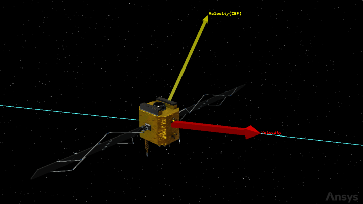
3D Graphics window VIEW
While you want your focus to be on the vector graphics, the display in the 3D Graphics window can be distracting: the satellite's orbit track, the lighting effects, the stars in the background, and other aspects of the 3D Graphics window can take away from the focus of your visualization. While you could customize the 3D Graphics window by
Viewing vector graphics in the 3D Attitude Graphics window
The
Opening the 3D Attitude Graphics window
Open the 3D Attitude Graphics window with the Satellite object.
- Right-click on Satellite () in the Object Browser.
- Select Satellite in the shortcut menu.
- Select New 3D Attitude Graphics Window (
 ) in the Satellite submenu.
 - Use your mouse to get a look at the satellite when the 3D Attitude Graphics window opens.
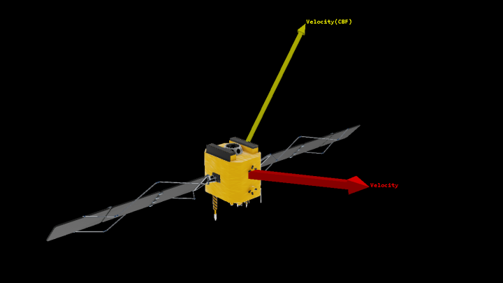
3D Attitude Graphics window VIEW
You can use your mouse to zoom and rotate in the 3D Attitude Graphics window just as you would in the 3D Graphics window. Note that the same components are simultaneously displayed for the satellite in the both the 3D Graphics and 3D Attitude Graphics windows.
Visualizing a plane
In addition to Vector components, you can also visualize Angles ( ), Axes (
 ), Points (
 ), and Planes (
 ) in the 3D Attitude Graphics window. Visualize the satellite’s body plane.
- Return to Satellite's () Properties ().
- Select the Planes tab.
- Select the Show check box for Body.XY Plane.
- Clear the Show Label check box.
- Enter 70 in the Translucent plane field.
- Click to confirm your changes and to keep the Properties Browser open.
- Bring the 3D Attitude Graphics window to the front.
- Return to Satellite's () Properties ().
- Clear the Show check box for Body.XY Plane.
- Click to confirm your change and to keep the Properties Browser open.
The Body X-Y plane refers to the X-Y quadrant of the satellite's Body axes.
The plane will be 70 percent transparent.
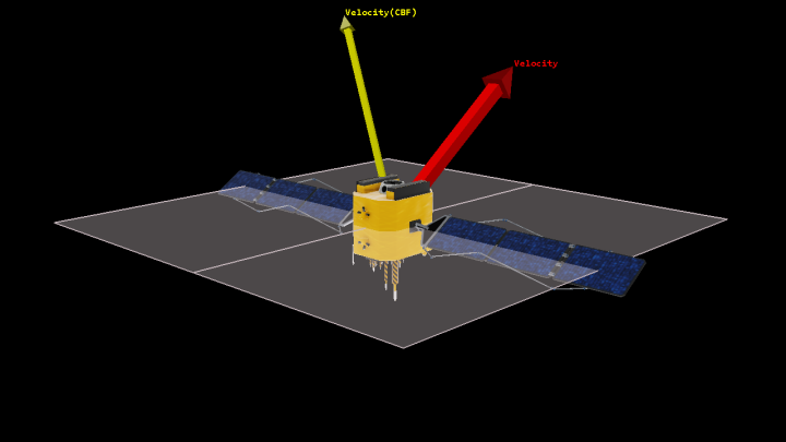
Body XY Plane
Note the plane's alignment with the body axes of the Satellite object.
Creating custom components with the Vector Geometry tool
The Analysis Workbench capability comprises four application-wide tools (the Vector Geometry tool, the Time tool, the Calculation tool, and the Spatial Analysis tool) that you can use to create custom components and insert them into your scenarios. They are designed to streamline, organize, and extend the fundamental computational capabilities of the STK software. You can use these tools to create components that suit your needs. The Vector Geometry tool creates geometry components with time-varying placement or orientation in 3D space, including Vectors ( ), Axes (), Points (), Systems (
 ), Angles (), and Planes ().
Opening the Analysis Workbench
Access the Vector Geometry tool by opening the Analysis Workbench.
- Right-click on Satellite () in the Object Browser.
- Select Analysis Workbench... (
 ) in the shortcut menu.
 - Select the Vector Geometry tab when the Analysis Workbench opens.
Creating a new Vector component
Create a velocity vector with the satellite body frame as its reference axes.
- Click Create new Vector () on the Vector Geometry toolbar.
- Click Type: when the Add Geometry Component dialog box opens.
- Select Derivative () in the Select Component Type list when the Select Component Type dialog box opens.
- Click to confirm your selection and to close the Select Component Type dialog box.
- Enter Velocity(Body) in the Name field.
This will create a derivative of a vector computed with respect to specified axes.
Viewing the base vector and reference axes
Take a look at the components that are selected for the vector and the reference axes.
- Click the Vector ellipsis (
 ).
). - Ensure Position (
 ) is selected in the Vectors for: Satellite tree when the Select Reference Vector dialog box opens.
 - Click to close the Select Reference Vector dialog box without making any changes.
- Click the Reference Axes ellipsis ().
- Ensure Body (
 ) is selected in the Aces for: Satellite tree when the Select Reference Axes dialog box opens.
 - Click to close the Select Reference Axes dialog box without making any changes.
- Click to confirm your changes and to close the Add Geometry Component dialog box.
Position () is a displacement vector between the Earth's center point and the Satellite's center point.
The value of the Derivative vector is computed using analytic formulas.
Viewing the vector's dependency tree
The Analysis Workbench's shortcut menu provides options to examine dependencies of the selected component, which opens a new dialog box with a
- Right-click on Velocity(Body) (), located in the My Components () folder in the Components for: Satellite tree.
- Select Show Dependencies... in the shortcut menu.
- Note the Show dependents option is selected when the Dependency Tree opens.
- Note that only Satellite/Satellite Velocity(Body) () is listed in the Dependencies for Satellite Velocity(Body) Vector tree.
- Select the Show constituents option.
- Expand (
 ) all the elements in the Dependencies for Satellite Velocity(Body) Vector tree.
 - Click to close the Dependency Tree.
- Click to close the Analysis Workbench.
Vector components you create are editable and are grouped in the My Components () folder.
The Show constituents option shows the reverse: everything on which the vector depends.
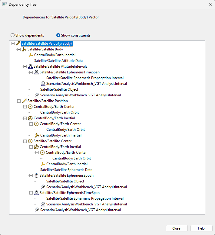
Velocity(Body) vector Dependency Tree
Note that there are a number of components that are automatically created when you created your Velocity(Body) vector.
Displaying the Velocity(Body) vector in the 3D Attitude Graphics window
Update the satellite's 3D Graphics - Vector properties to display the Velocity(Body) vector in the 3D Attitude Graphics window.
- Return to Satellite's () Properties ().
- Select the Vectors tab.
- Click .
- Select Velocity(Body) (), located in the My Components () folder in the Components for: Satellite tree, when the Add Components dialog box opens.
- Click to confirm your selection and to close the Add Components dialog box.
- Click to confirm your changes and to keep the Properties Browser open.
- Bring the 3D Attitude Graphics window to the front.
Vector_720x405.png)
Velocity(Body) vector
The new vector now appears in the 3D Attitude Graphics window.
Creating a new Angle component
In addition to vectors and planes, you can display angles in the 3D Graphics and 3D Attitude Graphics windows. Use the Vector Geometry tool to create a new angle component.
- Return to Satellite's () Properties ().
- Select the Angles tab.
- Click .
- Click Create new Angle () on the Vector Geometry toolbar when the Add Components dialog box opens.
- Leave the Type set to Between Vectors when the Add Geometry Component dialog box opens.
- Enter VelocityDifference in the Name field.
This type defines an angle between two vectors.
Selecting the angle's reference vectors
Choose the To and From vectors to define your Between Vectors angle.
- Click the From Vector ellipsis ().
- Select Velocity (), located in the Installed Components () folder in the Vectors for: Satellite tree, when the Select Reference Vector dialog box opens.
- Click to confirm your selection and to close the Select Reference Vector dialog box.
- Click the To Vector ellipsis ().
- Select Velocity(CBF) (), located in the Installed Components () folder in the Vectors for: Satellite tree, when the Select Reference Vector dialog box opens.
- Click to confirm your selection and to close the Select Reference Vector dialog box.
- Click to confirm your changes and to close the Add Geometry Component dialog box.
- Select VelocityDifference (), located in the My Components () folder in the Components for: Satellite tree.
- Click to confirm your changes and to close the Add Components dialog box.
Viewing the angle in the 3D Attitude Graphics window
Take a look at the angle in the 3D Attitude Graphics window.
- Ensure VelocityDifference Angle is selected in the list.
- Clear the Show label check box.
- Click to confirm your changes and to keep the Properties Browser open.
- Bring the 3D Attitude Graphics window to the front.
- Click Start () on the Animation toolbar.
- Observe the changes in the angle value as the vectors defining it move apart and back together.
- Click Reset (
 ) when finished.
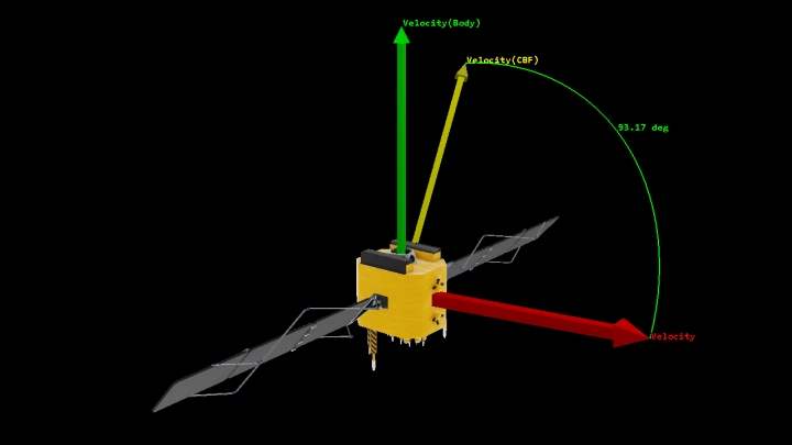
VelocityDifference Angle
Adding another new angle
Now that you know how to create and display angles, add another angle between the Velocity vector and the Velocity(Body) vector.
- Return to Satellite's () Properties ().
- Click .
- Click Create new Angle () on the Vector Geometry toolbar when the Add Components dialog box opens.
- Leave the Type set to Between Vectors when the Add Geometry Component dialog box opens.
- Enter Velocity(Body)Difference in the Name field.
Selecting the angle's reference vectors
Choose the To and From vectors to define your angle.
- Click the From Vector ellipsis ().
- Select Velocity (), located in the Installed Components () folder in the Vectors for: Satellite tree, when the Select Reference Vector dialog box opens.
- Click to confirm your selection and to close the Select Reference Vector dialog box.
- Click the To Vector ellipsis ().
- Select Velocity(Body) (), located in the My Components () folder in the Vectors for: Satellite tree, when the Select Reference Vector dialog box opens.
- Click to confirm your selection and to close the Select Reference Vector dialog box.
- Click to confirm your changes and to close the Add Geometry Component dialog box.
- Select Velocity(Body)Difference (), located in the My Components () folder in the Components for: Satellite tree.
- Click to confirm your changes and to close the Add Components dialog box.
Viewing the angle in the 3D Attitude Graphics window
Take a look at the angle in the 3D Attitude Graphics window.
- Ensure Velocity(Body)Difference Angle is selected in the list.
- Clear the Show label check box.
- Click to confirm your changes and to keep the Properties Browser open.
- Bring the 3D Attitude Graphics window to the front.
- Click Start () on the Animation toolbar.
- Observe the changes in the angles.
- Click Reset () when finished.
- Return to Satellite's () Properties ().
- Clear the Show check boxes for both VelocityDifference Angle and Velocity(Body)Difference Angle in the list.
- Click to confirm your changes and to keep the Properties Browser open.
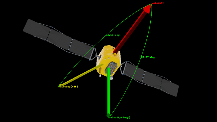
Velocity(Body)Difference Angle
Using the Attitude Sphere
The
Defining and displaying the attitude sphere
Update the satellite's 3D Graphics Attitude Sphere properties to display its attitude sphere.
- Select the 3D Graphics – Attitude Sphere page.
- Select the Show check box in the Attitude Sphere panel.
- Enter 0.700 in the Value field in the Scale panel.
- Note the Sphere Color and Grid line width options.
- Note the Zero Deg Color and Zero Deg line width options.
- Note Satellite VVLH is selected for the Frame.
- Note that Earth, Sun, and Moon are selected to show in the Projections list.
- Click to confirm your changes and to keep the Properties Browser open.
This is a logarithmic scaling factor for the sphere.
These control the appearance of the grid lines defining the sphere.
These options are used to highlight the equator and prime meridian lines as desired.
The Frame field lets you select a reference frame for the sphere display. In the VVLH (Vehicle Velocity Local Horizontal) frame, the axes align the Z axis opposite to the position vector and the X axis toward the inertial velocity vector.
The Projections list lets you control the display the projection of the position of central bodies and other objects of interest on the surface of the attitude sphere. You can use projections on the Attitude Sphere to help you analyze the velocity of a satellite relative to other bodies, such as the Earth.
Viewing the attitude sphere
As a representation of your reference frame, the Attitude Sphere may make it easier at times to understand the velocity, position, or attitude of an object. Take a look a the attitude sphere in the 3D Attitude Graphics window.
- Bring the 3D Attitude Graphics window to the front.
- Use your mouse to zoom out to get a better view of the Attitude Sphere around Satellite.
- Click Start () on the Animation toolbar.
- As the scenario animates, notice a blue circle that changes in size on the surface of the sphere.
- Note the comparative sizes of the projections of the Sun and Moon.
- Click Reset () when finished.
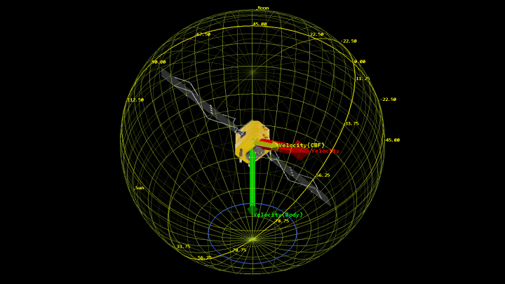
Attitude Sphere
This is the projection of the Earth.
Unlike the Earth, the Sun and Moon projections are labeled. All three projections provide situational awareness of where they are located in respect to Satellite. For instance, if you were to draw a straight line from the center point of Satellite to the center point of the Sun, that line would pass through the middle of the Sun projection at all times.
Showing projection volume graphics
You can also display a projection in three dimensions.
- Return to Satellite's () Properties ().
- Select the Volume check box for Earth in the Projections panel list.
- Click to confirm your selection and to keep the Properties Browser open.
- Bring the 3D Attitude Graphics window to the front.
- Click Start () on the Animation toolbar.
- Click Pause () when the satellite is at apogee.
- Click Reset () when finished.
- Return to Satellite's () Properties ().
- Clear the Show check box for the attitude sphere to turn off its display.
- Click to confirm your change and to keep the Properties Browser open.
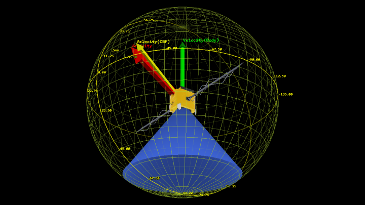
Attitude Sphere volume graphics
The Earth's projection is now displayed as a cone.
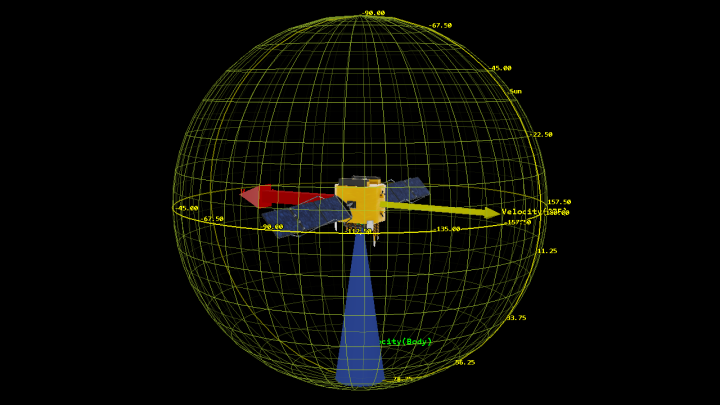
Attitude Sphere Vector graphics near apogee
At apogee, the Earth-defined vectors (Velocity and Velocity(CBF)) will appear at approximate right angles to the Earth projection cone, as would be expected.
Creating a persistent vector display
Use vector persistence options to control the way in which geometric elements appear in the 3D Graphics window as the animation time elapses and the position of those elements change.
Opening the 3D Graphics - Vector properties
You can set the vector persistence graphics on the satellite's 3D Graphics - Vector page.
- Select the 3D Graphics - Vector page.
- Select the Vectors tab.
Selecting the reference axes
Use the ICRF (International Celestial Reference Frame) for the axes that define the coordinate frame to which the display options are applied for the Velocity(CBF) and Velocity(Body) vectors. The International Celestial Reference Frame axes are defined as the inertial (i.e., kinematically nonrotating) axes associated with a general relativity frame centered at the solar system barycenter (often called the BCRF). The IAU (International Astronomical Union) is the authority for the definition of the ICRF. The ICRF is the best realization of an inertial frame constructed to date and thus represents an improvement upon the theory behind the J2000 frame. While the ICRF and J2000 frames themselves are very close, they are not identical; moreover, the J2000 frame rotates (very slowly) over time with respect to the ICRF frame. Recent star catalogs and celestial body ephemerides are most often expressed natively with respect to the ICRF frame.
- Clear the Show check box for Velocity(Body) Vector in the list.
- Select Velocity Vector in the list.
- Click the Axes ellipsis ().
- Select ICRF (
 ), located in the Installed Components () folder in the Axes for: Satellite tree, when the Select Reference Axes dialog box opens.
 - Click to confirm your selection and to close the Select Reference Axes dialog box.
- Select Velocity(CBF) Vector in the list.
- Click the Axes ellipsis ().
- Select ICRF (), located in the Installed Components () folder in the Axes for: Satellite tree, when the Select Reference Axes dialog box opens.
- Click to confirm your selection and to close the Select Reference Axes dialog box.
Setting the persistence options
Set the options to successively display geometric elements over a specified duration.
- Select Velocity Vector in the list.
- Select the Show check box in the Persistence panel.
- Select the Fade check box.
- Enter 1 day in the Duration field.
- Note that Sweep is selected for the Connect option by default.
- Select Velocity(CBF) Vector in the list.
- Select the Show check box in the Persistence panel.
- Select the Fade check box.
- Enter 1 day in the Duration field.
- Click to confirm your changes and to close the Properties Browser.
When selecting the Fade option, earlier occurrences of a geometric element display will fade over time so that it is drawn as completely filled at the most recent animation time and fades as the animation moves forward.
This sets the length of time during which the geometric element is visible.
When Sweep is selected, a continuous band of color representing the path of the element will be shown.
Viewing the changes in the 3D Graphics window
View the changes in the 3D Graphics (not the 3D Attitude Graphics) window.
- Bring the 3D Graphics window to the front.
- Click Start () on the Animation toolbar.
- Click Reset () when finished.
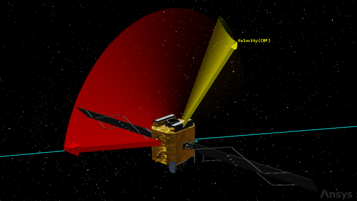
Persistent vector graphics
Watch as the two velocity vectors sweep out their respective disks.
Changing the view direction
Update the
- Click View From/To (
 ) on the 3D Graphics window's 3D Graphics toolbar.
 - Select the Along a Direction option when the View From/To dialog box opens.
- Ensure Satellite () is selected in the From Position list.
- Click Add Vector () in the Direction panel.
- Select Velocity (), located in the Installed Components () folder in the Vectors for: Satellite tree, when the Select Vector dialog box opens.
- Click to confirm your selection and to close the Select Vector dialog box.
- Select the Inward option.
- Click to confirm your changes and to close the View From/To dialog box.
Using the Along a Direction viewing mode, you can set the view along an existing vector or a vector created in the Vector Geometry Tool.
Selecting the Inward option will reverse the 'view from' position and the 'view direction'.
Viewing the changes in the 3D Graphics window
Animate your scenario to see the changes.
- Click Start () on the Animation toolbar.
- Use the mouse to rotate the view around the satellite.
- Note that the Velocity vector sweeps out a flat disk while the Velocity(CBF) vector sweeps out a warped disk.
- Watch as the satellite descends through its orbit.
- Click Reset () when finished.
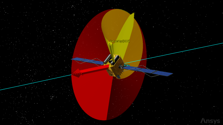
Persistent vector graphics in another reference frame
This is expected, as these disks are drawn in an inertial frame.
Recall that the satellite you created at the beginning of this tutorial in a Molniya orbit. On the descending side of its orbit, its motion relative to the rotating Earth is in the opposite direction to its motion on the ascending side. The motion of a vector defined in a CBF framework will reflect this difference.
Saving your work
Clean up and close out your scenario.
- Close any open tools and properties.
- Save () your work.
Summary
You began by inserting a notional Satellite object in a Molniya orbit. You used the Analysis Workbench capability's Vector Geometry tool, in conjunction with the satellite's 3D Graphics - Vector properties to display several built-in Vector Geometry components and to create and display custom Vector and Angle components in the 3D Attitude Graphics window. You explored the attitude sphere and its capabilities before exploring vector persistence graphics in the 3D Graphics window. Using the Vector Geometry tool, you were able to visualize the differences among vectors defined in different reference frames.