STK Premium (Space) or STK Enterprise
You can obtain the necessary licenses for this tutorial by contacting AGI Support at support@agi.com or 1-800-924-7244.
The results of the tutorial may vary depending on the user settings and data enabled (online operations, terrain server, dynamic Earth data, etc.). It is acceptable to have different results.
The technical notes for this exercise can be viewed here.
Capabilities covered
This lesson covers the following capabilities of the Ansys Systems Tool Kit® (STK®) digital mission engineering software:
- STK Pro
- Astrogator
Problem statement
Engineers and operators want to transfer a satellite from a low Earth orbit (LEO) in a circular parking orbit with a radius of 6,570 kilometers and an inclination of 28 degrees to a geosynchronous orbit (GEO) with a radius of 42,160 kilometers and an inclination of zero.
This exercise is based on an example discussed in Sellers, Jerry Jon, Understanding Space: An introduction to Astronautics, New York: McGraw-Hill (1994), pp. 191-192.
Solution
Use the STK/Astrogator® capability to design a Hohmann transfer to increase the radius of the orbit, followed by a maneuver to decrease its inclination. Then, perform the second phase of the Hohmann transfer together with the inclination change in a combined maneuver to compare the economy of the two methods.
What you will learn
Upon completion of this tutorial, you will be able to:
- Design a simple Hohmann transfer followed by an inclination change
- Design a combined Hohmann transfer followed by an inclination change
- Maximize the efficiency of orbital plane changes
Video guidance
Watch the following video. Then follow the steps below, which incorporate the systems and missions you work on (sample inputs provided).
Creating a new scenario
First, you must create a new scenario, and then build from there.
- Launch the STK application (
 ).
). - Click
 Create a Scenario when the Welcome to STK dialog box opens.
 - Enter the following in the STK: New Scenario Wizard:
- Click when you finish.
- Click Save (
 ) when the scenario loads.
 - Verify the scenario name and location in the Save As dialog box.
- Click .
| Option | Value |
|---|---|
| Name | Inclination_Plane_Change |
| Start | 1 Sep 2025 16:00:00.000 UTCG |
| Stop | + 3 days |
The STK application creates a folder with the same name as your scenario for you.
Save (![]() ) often during this scenario!
) often during this scenario!
Cleaning up your workspace
The Timeline View and the 2D Graphics window aren't needed in this scenario.
- Close (
 ) the 2D Graphics window.
 - Close () the Timeline View.
Inserting a Satellite object
Insert a Satellite object.
- Bring the Insert STK Objects tool (
 ) to the front.
 - Select Satellite (
 ) in the Select An Object To Be Inserted list.
 - Select Insert Default () in the Select A Method list.
- Click .
- Right-click on Satellite1 () in the Object Browser.
- Select Rename in the shortcut menu.
- Rename Satellite1 () Sat_PlaneChange.
Setting the 3D Graphics Pass properties
Choose how you want to display the Satellite object's orbit in the 3D Graphics window on the
- Right-click on Sat_PlaneChange () in the Object Browser.
- Select Properties (
 ) in the shortcut menu.
 - Select the 3D Graphics - Pass page when the Properties Browser opens.
- Open the Lead Type drop-down list in the Orbit Track panel.
- Select All.
- Click to confirm your changes and to keep the Properties Browser open.
The Lead Type defines the display of the leading portion of a vehicle's track. Selecting All displays the track spanning the entirety of the vehicle's ephemeris.
Changing the propagator to Astrogator
The
- Select the Basic - Orbit page.
- Open the Propagator drop-down list.
- Select Astrogator.
- Click to confirm your selection and to keep the Properties Browser open.
Setting up the Mission Control Sequence
The Mission Control Sequence (MCS) is the core of your space mission scenario. The MCS functions as a graphical programming language, in which mission segments dictate how Astrogator calculates the trajectory of the spacecraft based on the general settings that you specify for the MCS itself.
The MCS is defined by selecting and organizing MCS Segments in a manner that produces your desired trajectory. The left side of the MCS is represented schematically by a tree structure, which lists the segments that make up the MCS and depicts their relationships to each other. Above the tree is the MCS toolbar, which contains buttons that perform various MCS and individual segment operations. By default, the MCS contains Initial State and Propagate segments that produce a low Earth orbit. The right side of the window contains the parameters of the segment that is currently selected in the MCS Tree.
Defining the Initial State segment
Use the
- Right-click on Initial State (
 ) in the MCS.
 - Select Rename in the shortcut menu.
- Rename Initial State () 28 deg Inclined Orbit.
Defining the Initial State segment elements
Specify the state at a given epoch in a variety of coordinate types and in any coordinate system. You will use the Keplerian coordinate system. The Classical coordinate type uses the traditional osculating Keplerian orbital elements to specify the shape and size of an orbit.
- Select the Elements tab.
- Open the Coordinate Type drop-down list.
- Select Keplerian.
- Set the following orbital parameters:
- Leave the remaining default values.
- Click to confirm your changes and to keep the Properties Browser open.
| Option | Value |
|---|---|
| Semi-major Axis | 6570 km |
| Inclination | 28 deg |
Setting the fuel tank configuration
Set the maximum fuel mass and the fuel mass of the
- Select the Fuel Tank tab.
- Enter the following values:
- Click to confirm your changes and to keep the Properties Browser open.
| Option | Value |
|---|---|
| Maximum Fuel Mass | 5000 kg |
| Fuel Mass | 5000 kg |
Propagating the parking orbit
Use the
- Select Propagate (
 ) in the MCS.
 - Rename Propagate () Propagate 2 Hours.
Setting the stopping condition
- Look in the Stopping Conditions panel.
- Notice that the default stopping condition for the Propagate 2 Hours Propagate segment is Duration.
- Enter 7200 sec in the Trip field.
- Click to confirm your changes and to keep the Properties Browser open.
7200 seconds, or 2 hours, is more than enough time to have the satellite orbit one complete pass.
Adding a Target Sequence
Add a
- Select Propagate 2 Hours () in the MCS.
- Click Insert Segment After (
 ) in the MCS toolbar.
 - Select Target Sequence (
 ) in the Segment Selection dialog box.
 - Click to confirm your selection and to close the Segment Selection dialog box.
- Rename Target Sequence () Begin Hohmann Transfer.
- Click to confirm your changes and to keep the Properties Browser open.
Inserting an Impulsive Maneuver segment
For an
- Right-click on the Return (
 ) segment that's nested within Begin Hohmann Transfer ().
 - Select Insert Before... in the shortcut menu.
- Select Maneuver (
 ) in the Segment Selection dialog box.
 - Click to confirm your selection and to close the Segment Selection dialog box.
- Notice that the default Maneuver Type is Impulsive.
Changing the segment properties
Rename the Maneuver segment.
- Rename Maneuver () DV1.
- Click to confirm your change and to keep the Properties Browser open.
DV simply stands for Delta-V.
Viewing the maneuver's attitude control
The Attitude Control field enables you to select the mode in which the maneuver pointing direction is prescribed. Use the default Attitude Control setting of Along Velocity Vector. The satellite object’s attitude is such that the Delta-V vector aligns with the spacecraft's inertial velocity vector. The inertial reference frame depends on the central body of the satellite object. Either the thruster set or an engine model defines the Delta-V in the body frame.
- Select the Attitude tab.
- Notice that the Attitude Control defaults to Along Velocity Vector.
Selecting the independent variable
A Target Sequence's differential corrector profile uses a differential correction algorithm to achieve a goal value or set of values. The values that the profile targets are called independent variables, or control parameters. The values that define the goal of the profile are called dependent variables, or equality constraints (or results). When the Target Sequence runs, it will change the values of the independent variables to achieve the goal. You can use any element of a nested MCS segment or linked component as an independent variable. Use Delta-V Magnitude which is the magnitude of the impulse to be added to the spacecraft velocity vector in distance / time.
- Click on the Delta-V Magnitude target (
 ).
). - Notice the target now has a check mark (
 ).
).
Selecting the target makes Delta-V Magnitude an independent variable. This tells Astrogator to determine the Delta-V based on user determined results.
Updating mass based on fuel usage
Set DV1 to update the satellite's mass based on its fuel usage.
- Select the Engine tab.
- Select the Update Mass Based on Fuel Usage check box.
- Click to confirm your changes and to keep the Properties Browser open.
Selecting the results component
Dependent variables for a differential corrector profile are defined in terms of calculation objects. For DV1, select Radius Of Apoapsis for the calculation object.
- Click at the bottom of the MCS.
- Expand (
 ) the Keplerian Elems (
 ) folder in the Available Components list when the User - Selected Results - DV1 dialog box opens.
 - Select Radius Of Apoapsis (
 ).
). - Click Insert Component (
 ) to move Radius Of Apoapsis () to the selected components list.
 - Click to close the User - Selected Results - DV1 dialog box.
- Click to confirm your changes and to keep the Properties Browser open.
Setting up the differential corrector profile
You can configure a Target sequence to execute in many different ways depending on the solution you are trying to achieve. Set up the differential corrector profile to change the Delta-V Magnitude to achieve the desired radius of apoapsis.
- Select Begin Hohmann Transfer () in the MCS.
- Open the Action drop-down list.
- Select Run active profiles.
Selecting Run active profiles allows the active profiles to operate when you run the Mission Control Sequence.
Setting the independent variable
Use Delta-V Magnitude as the control parameter (independent variable).
- Select Differential Corrector in the Profiles panel.
- Click Properties... () in the Profiles toolbar.
- Select the Use check box for ImpulsiveMnvr.Pointing.Spherical.Magnitude in the Control Parameters panel when the Differential Corrector dialog box opens.
Setting the dependent variable
Use the radius of apoapsis as the equality constraint (result) with a goal of 42,160 kilometers. Astrogator will use the specified radius of apoapsis to determine the required Delta-V. No change in inclination will be attempted in this maneuver.
- Select the Use check box for Radius_Of_Apoapsis in the Equality Constraints (Results) panel.
- Click on the Desired Value cell.
- Enter 42160 km in the Desired Value cell.
- Click to confirm your selections and to close the Differential Corrector dialog box.
- Click to confirm your changes and to keep the Properties Browser open.
Inserting a Propagate segment
Insert a new Propagate segment.
- Right-click on the bottommost Return () segment in the MCS.
- Select Insert Before... in the shortcut menu.
- Select Propagate () in the Segment Selection dialog box.
- Click to confirm your selection and to close the Segment Selection dialog box.
Changing the segment properties
Change the name and color of the Propagate segment.
- Select Propagate () in the MCS.
- Click Segment Properties () in the MCS toolbar.
- Enter Prop to Apogee in the Name field of the Edit Segment dialog box.
- Open the Color drop-down list.
- Select a color that's different from Propagate 2 Hours ().
- Click to confirm your changes and to close the Edit Segment dialog box.
- Click to confirm your changes and to keep the Properties Browser open.
Propagate segments can be viewed in the 3D Graphics window. By changing the color of each Propagate segment (if you have multiple Propagate segments), you can view them visually. You configured the 3D Graphics Pass properties so that the Maneuver segments nested within the Target Sequences won't be visible in the 3D Graphics window when you propagate the satellite.
Inserting an apoapsis stopping condition
Use the apoapsis stopping condition to stop at the farthest point from the origin.
- Click New... (
 ) in the Stopping Conditions panel toolbar.
 - Select Apoapsis () in the New Stopping Condition dialog box.
- Click to confirm your selection and to close the New Stopping Condition dialog box.
- Select the Duration stopping condition.
- Click Delete (
 ) in the stopping conditions toolbar.
 - Click to confirm your changes and to keep the Properties Browser open.
Adding a second Target Sequence
In this Target Sequence, you will calculate the Delta-V required to circularize the orbit; that is, change its eccentricity to zero. Again, no change in inclination will be targeted.
- Select Prop to Apogee () in the MCS.
- Click Insert Segment After () in the MCS toolbar.
- Select Target Sequence () in the Segment Selection dialog box.
- Click to confirm your selection and to close the Segment Selection dialog box.
- Rename Target Sequence () Finish Hohmann Transfer.
Inserting an Impulsive Maneuver segment
Add an Impulsive Maneuver segment to the Finish Hohmann Transfer Target Sequence.
- Right-click on the Return () segment that's nested within Finish Hohmann Transfer ().
- Select Insert Before... in the shortcut menu.
- Select Maneuver () in the Segment Selection dialog box.
- Click to confirm your selection and to close the Segment Selection dialog box.
Changing the segment properties
Change the name of the Maneuver segment.
- Rename Maneuver () DV2.
- Click to confirm your change and to keep the Properties Browser open.
Setting the satellite's independent variable
Select Delta-V Magnitude as an independent variable for DV2.
- Select the Attitude tab.
- Select the Delta-V Magnitude as the independent variable ().
Updating mass based on fuel usage
Like with DV1, set DV2 to update the satellite's mass based on its fuel usage.
- Select the Engine tab.
- Select the Update Mass Based on Fuel Usage check box.
- Click to confirm your changes and to keep the Properties Browser open.
Selecting the results component
Use Eccentricity for DV2's calculation object.
- Click at the bottom of the MCS.
- Expand () the Keplerian Elems () folder in the Available Components list when the User - Selected Results - DV2 dialog box opens.
- Select Eccentricity ().
- Click Insert Component () to move Eccentricity () to the selected components list.
- Click to close the User - Selected Results - DV2 dialog box.
- Click to confirm your changes and to keep the Properties Browser open.
Setting up the differential corrector profile
Set your Mission Control Sequence to Run active profiles to allow the active profiles to operate.
- Select Finish_Hohmann_Transfer () in the MCS.
- Open the Action drop-down list.
- Select Run active profiles.
Setting the independent variable
Use Delta-V Magnitude as the control parameter (independent variable).
- Select Differential Corrector in the Profiles panel.
- Click Properties... () in the Profiles toolbar.
- Select the Use check box for ImpulsiveMnvr.Pointing.Spherical.Magnitude in the Control Parameters panel when the Differential Corrector dialog box opens.
Setting the dependent variable
Use eccentricity as the equality constraint (result) with a zero (0) kilometer desired value, targeting a circular orbit.
- Select the Use check box for Eccentricity in the Equality Constraints (Results) panel.
- Keep the Desired Value setting of 0 (zero).
- Enter 0.001 in the Tolerance field.
- Click to confirm your selections and to close the Differential Corrector dialog box.
- Click to confirm your changes and to keep the Properties Browser open.
Inserting a Propagate segment
Insert a new Propagate segment. To carry out a plane change to zero inclination, the satellite must be at ascending or descending node. Propagate it to ascending node.
- Right-click on the bottommost Return () segment in the MCS.
- Select Insert Before... in the shortcut menu.
- Select Propagate () in the Segment Selection dialog box.
- Click to confirm your selection and to close the Segment Selection dialog box.
Changing the segment properties
Change the name and color of the Propagate segment.
- Select Propagate () in the MCS.
- Click Segment Properties () in the MCS toolbar.
- Enter Prop to Ascending Node in the Name field of the Edit Segment dialog box.
- Open the Color drop-down list.
- Select a color that's different from the other Propagate () segments.
- Click to confirm your changes and to close the Edit Segment dialog box.
- Click to confirm your changes and to keep the Properties Browser open.
Inserting an ascending node stopping condition
Use the ascending node stopping condition to stop when crossing the X-Y plane from the south to the north.
- Click New... () in the Stopping Conditions panel toolbar.
- Select AscendingNode () in the New Stopping Condition dialog box.
- Click to confirm your selection and to close the New Stopping Condition dialog box.
- Select the Duration stopping condition.
- Click Delete () in the stopping conditions toolbar.
- Enter 2 in the Repeat Count field.
- Click to confirm your changes and to keep the Properties Browser open.
The satellite will make at least one complete orbit pass (and one will be drawn in the 3D Graphics window) before the plane change maneuver is executed.
Adding a Target sequence
Here, you will calculate the Delta-V required to maneuver the satellite into an orbit with an inclination of zero degrees.
- Select Prop to Ascending Node () in the MCS.
- Click Insert Segment After () in the MCS toolbar.
- Select Target Sequence () in the Segment Selection dialog box.
- Click to confirm your selection and to close the Segment Selection dialog box.
- Rename Target Sequence () Simple Plane Change.
- Click to confirm your changes and to keep the Properties Browser open.
Inserting an Impulsive Maneuver segment
Add an Impulsive Maneuver segment to the Simple Plane Change Target Sequence.
- Right-click on the Return () segment that's nested within Simple Plane Change ().
- Select Insert Before... in the shortcut menu.
- Select Maneuver () in the Segment Selection dialog box.
- Click to confirm your selection and to close the Segment Selection dialog box.
Changing the segment properties
Change the name of the Maneuver segment.
- Rename Maneuver () DV3.
- Click to confirm your change and to keep the Properties Browser open.
Selecting the independent variables
Use Thrust Vector as the attitude control setting. With this attitude control setting, you specify the Delta-V vector in some reference frame using either Cartesian or spherical components. Astrogator then computes the attitude so that the total thrust vector in the body frame, as specified by the thruster set or engine model, aligns with this vector in the reference axes. Select the Delta-V vector's Cartesian X (Velocity) and Y (Normal) as the independent variables.
- Select the Attitude tab.
- Open Attitude Control drop-down list.
- Select Thrust Vector.
- Select X (Velocity) as an independent variable ().
- Select Y (Normal) as an independent variable ().
- Click to confirm your changes and to keep the Properties Browser open.
The thrust vector describes the direction of acceleration applied to a satellite. This direction is opposite to the exhaust of an engine. For example, for a single chemical rocket engine mounted to a satellite, the thrust vector is opposite to the direction of the center of the exhaust plume flames. If the satellite uses more than one engine together in a thruster set, the thrust vector is along the direction of the combined effective acceleration. This direction is determined by calculating the sum of the acceleration vectors of each individual thruster.
Updating mass based on fuel usage
As with DV1 and DV2, set DV3 to update the satellite's mass based on its fuel usage.
- Select the Engine tab.
- Select the Update Mass Based on Fuel Usage check box.
- Click to confirm your changes and to keep the Properties Browser open.
Selecting the results components
In this instance, you will use the inclination and eccentricity components for DV3's calculation objects.
- Click at the bottom of the MCS.
- Expand () the Keplerian Elems () folder in the Available Components list when the User - Selected Results - DV3 dialog box opens.
- Select Eccentricity ().
- Click Insert Component () to move Eccentricity () to the selected components list.
- Select Inclination ().
- Click Insert Component () to move Inclination () to the selected components list.
- Click to close the User - Selected Results - DV3 dialog box.
- Click to confirm your changes and to keep the Properties Browser open.
Setting up the differential corrector profile
Set your Mission Control Sequence to Run active profiles to allow the active profiles to operate.
- Select Simple Plane Change () in the MCS.
- Open the Action drop-down list.
- Select Run active profiles.
Setting the independent variables
Use the Delta-V vector's Cartesian X (Velocity) and Y (Normal) as the Control Parameters (independent variables).
- Select Differential Corrector in the Profiles panel.
- Click Properties... () in the Profiles toolbar.
- Select the Use check box for ImpulsiveMnvr.Pointing.Cartesian.X in the Control Parameters panel when the Differential Corrector dialog box opens.
- Select the Use check box for ImpulsiveMnvr.Pointing.Cartesian.Y.
Setting the dependent variables
Set Eccentricity and Inclination as the equality constraints (results) for the Simple Plane Change Target Sequence.
- Select the Use check box for Eccentricity in the Equality Constraints (Results) panel.
- Enter 0.001 in the Tolerance field.
- Select the Use check box for Inclination.
- Leave the desired value set to 0 deg.
- Click to close the Differential Corrector dialog box.
- Click to confirm your changes and to keep the Properties Browser open.
The profile will stop when it achieves a value within this range of the Desired Value.
Inserting a Propagate segment
Add a new Propagate segment after the Simple Plane Change Target Sequence.
- Right-click on the bottommost Return () segment in the MCS.
- Select Insert Before... in the shortcut menu.
- Select Propagate () in the Segment Selection dialog box.
- Click to confirm your selection and to close the Segment Selection dialog box.
Changing the segment properties
Change the name and color of the Propagate segment.
- Select Propagate () in the MCS.
- Click Segment Properties () in the MCS toolbar.
- Enter Propagate 36 Hours in the Name field of the Edit Segment dialog box.
- Open the Color drop-down list.
- Select a color that's different from the other Propagate () segments.
- Click to confirm your changes and to close the Edit Segment dialog box.
- Click to confirm your changes and to keep the Properties Browser open.
Setting the stopping condition
Use a Duration stopping condition for the Propagate segment.
- Enter 36 hr in the Trip field.
- Click to confirm your changes and to keep the Properties Browser open.
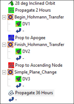
completed mcs view
Running the entire Mission Control Sequence
To calculate the trajectory of the spacecraft you must run the Mission Control Sequence. Astrogator will proceed through the MCS and run each segment, generating an ephemeris for the spacecraft. As it runs the MCS, Astrogator carries the trajectory and state of the spacecraft determined so far from one segment to the next.
- Click Run Entire Mission Control Sequence (
 ) in the MCS toolbar.
 - Click Clear Graphics (
 ) in the MCS toolbar.
 - Look at the Targeting Status windows.
- Close the Targeting Status windows.
- Click to close the Properties Browser.
- Save () your work.
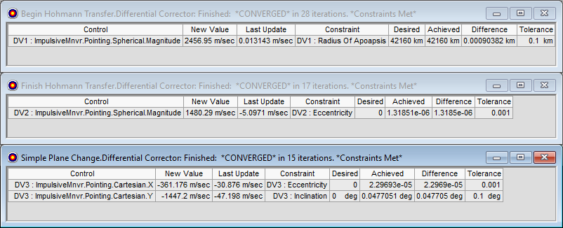
targeting status windows
Each maneuver and their results have a target status window showing the independent variables and results. The Delta-V required for each maneuver in seen in the New Value column.
The values you observe will differ slightly from those shown here, owing to minor differences in the scenario
The Delta-V required for the plane change is given by:
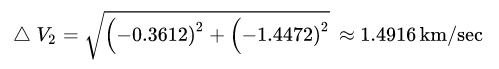
Thus, the total Delta-V (ΔVT) is:

As shown in the technical notes, in terms of the Delta-V required, this combination of maneuvers, in which a simple plane change is carried out at apogee of the transfer orbit, is less expensive than one in which the plane change occurs at perigee, but more expensive than one in which the plane change is combined with the second burn of the Hohmann Transfer.
Viewing the maneuvers in the 3D Graphics window
You can view each maneuver and its associated propagate stopping condition in the 3D Graphics window. You should see the colors that you set for each Propagate segment.
- Bring the 3D Graphics window to the front.
- Use your mouse to obtain a good view of all the maneuvers.
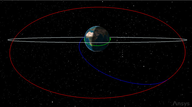
change from 28 to 0 degrees inclination
The orbit is circular before and after the inclination change. The final orbit is equatorial (has an inclination of zero).
Creating a Maneuver Summary report
Now that you have modeled the satellite's orbit and visualized its behavior, examine the results with a Maneuver Summary report.
- Right-click on Sat_PlaneChange () in the Object Browser.
- Select Report & Graph Manager... (
 ) in the shortcut menu.
 - Select the Maneuver Summary (
 ) report in the Installed Styles () folder in the Styles panel.
 - Click .
- Scroll through the Maneuver Summary report to view the amount of fuel used.
- Close the report and the Report & Graph Manager when you are finished viewing the data.
![]()
Separate Hohmann transfer and Inclination change fuel used
In defining the Initial State, you set the Fuel Mass to 5,000 kilograms. Take note of the total fuel used (for example, approximately 4,251 kg) for the three maneuvers.
Creating a combined inclination change
Combine the inclination change with the second burn of the Hohmann Transfer. One way to do this is to constrain the second Target sequence in terms of both inclination and eccentricity — that is, equatorializing and circularizing the orbit in the same maneuver.
Reusing the existing Satellite object
Instead of building a new Satellite object from scratch, you can adapt the one you just created.
- Select Sat_PlaneChange () in the Object Browser.
- Click Copy (
 ) in the Object Browser toolbar.
 - Click Paste (
 ) in the Object Browser toolbar.
 - Clear the Sat_PlaneChange () check box in the Object Browser.
The STK application automatically renames the copied object to Sat_PlaneChange1.
Resetting the Target Sequences
In order to use the existing segments and sequences in the MCS, some deletions and resets are required.
- Open Sat_PlaneChange1's () Properties ().
- Select the Basic - Orbit page when the Properties Browser opens.
- Select Begin Hohmann Transfer () in the MCS.
- Click in the Profiles and Corrections panel.
- Perform steps 3 and 4 for Finish Hohmann Transfer () and Simple Plane Change () in turn.
- Rename Simple Plane Change () Combined Change.
This will reset the controls of the search profiles to the nested segments' values.
Updating or deleting the MCS segments
You can reuse the existing segments from your first satellite, although you don't need all of them.
- Select Propagate 2 Hours () in the MCS.
- Click Delete Segment () in the MCS toolbar.
- Click to confirm.
- Click and drag Prop to Ascending Node () below 28 deg Inclined Orbit ().
- Rename DV1 () Simple DV.
- Delete () Finish Hohmann Transfer ().
- Click to confirm.
- Rename DV3 () Combined DV.
- Click to confirm your changes and to keep the Properties Browser open.
The nested DV2 (![]() ) Maneuver will automatically be deleted at the same time as the Target sequence.
) Maneuver will automatically be deleted at the same time as the Target sequence.
When you are finished, your MCS should look like the following:
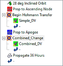
redesigned mcs
Ensuring the Simple DV Maneuver segment parameters are correct
Confirm that Simple DV is properly configured for your Hohmann transfer change.
- Select Simple DV () in the MCS.
- Verify that Delta-V Magnitude is selected as the independent variable ().
- Click .
- Verify that Radius Of Apoapsis () is selected as the elected component in the User Selected Results - Simple DV dialog box.
- Click to close the Select User Selected Results - Simple DV dialog box.
Ensuring the Combined DV Maneuver segment parameters are correct
Confirm that Combined DV is properly configured to change both the eccentricity and inclination in one maneuver.
- Select Combined DV () in the MCS.
- Verify that both X (Velocity) and Y (Normal) are selected as the independent variables ().
- Click .
- Verify that Eccentricity () and Inclination () are the selected components in the User Selected Results - Combined DV dialog box.
- Click to close the Select User Selected Results - Combined DV dialog box.
- Click to confirm your changes and to keep the Properties Browser open.
Verifying the Begin Hohmann Transfer Target sequence parameters are correct
Confirm that the Begin Hohmann Transfer Target Sequence is set to use the correct dependent and independent variables.
- Select Begin Hohmann Transfer () in the MCS.
- Click Properties... () in the Profiles panel toolbar.
- Verify that the Use check box is selected for ImpulsiveMnvr.Pointing.Spherical.Magnitude in the Control Parameters panel in the Differential Corrector dialog box.
- Verify that the Use check box is selected for Value for Radius_Of_Apoapsis.
- Verify that the Desired Value for Radius_Of_Apoapsis is set to 42160 km.
- Click to close the Differential Corrector dialog box.
Verifying the Combined Change Target sequence parameters are correct
Confirm that the Combined Change Target Sequence is set to use the correct dependent and independent variables.
- Select Combined Change () in the MCS.
- Click Properties... () in the Profiles panel toolbar.
- Verify that the Use check boxes in the Control Parameters panel for ImpulsiveMnvr.Pointing.Cartesian.X and ImpulsiveMnvr.Pointing.Cartesian.Y are selected in the Differential Corrector dialog box.
- Verify that the Use check boxes in the Equality Constraints (Results) panel for Eccentricity and Inclination are selected.
- Verify that the Desired Value for Eccentricity is set at 0 and the Tolerance is set at 0.001.
- Verify that the Desired Value for Inclination is set at 0 deg.
- Select the Convergence tab.
- Enter 100 in the Maximum Iterations field.
- Click to confirm your changes and to close the Differential Corrector dialog box.
This property defines the maximum number of evaluations that the profile will execute. If the profile does not reach the Desired Value, it will stop after the last iteration.
Running the entire Mission Control Sequence
With your Mission Control Sequence configured for a combined eccentricity and inclination change, run the entire MCS to propagate the satellite.
- Click Run Entire Mission Control Sequence () in the MCS toolbar.
- Click Clear Graphics () in the MCS toolbar.
- Click to confirm your changes and to keep the Properties Browser open.
- Look at the Targeting Status window.
- Close the Targeting Status windows.
- Click to close the Properties Browser.
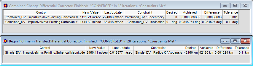
combined inclination change targeting status windows
The values you observe will differ slightly from those shown here, owing to minor differences in the scenario
Again, look at each targeting profile and observe the Final Values assigned to the control variables. The approximate Delta-V for the combined eccentricity and inclination change is:
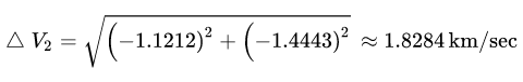
The total Delta-V (ΔVT) for the transfer from the low Earth, inclined parking orbit to the equatorial outer orbit is:

Due to the spatial geometry of the combined inclination change maneuver, its total Delta-V is less than the amount calculated for a Hohmann transfer followed by a separate plane change. See the
Viewing the maneuvers in the 3D Graphics window
You can view each maneuver and its associated propagate stopping condition in the 3D Graphics window. You should see the colors that you set for each Propagate segment.
- Bring the 3D Graphics window to the front.
- Use your mouse to obtain a good view of all the maneuvers.
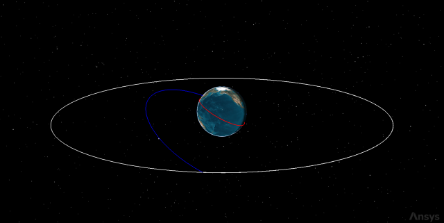
Combined Inclination change
The orbital and planar transfers occur as part of the same procedure.
Creating a Maneuver Summary report
Examine the results with a Maneuver Summary report and compare it to the previous plane change.
- Right-click on Sat_PlaneChange1 () in the Object Browser.
- Select Report & Graph Manager... () in the shortcut menu.
- Select the Maneuver Summary () report in the Installed Styles () folder in the Styles panel.
- Click .
- Scroll through the Maneuver Summary report.
![]()
Combined Inclination and plane change fuel used
Note the amount of fuel used (for example, approximately 3,873 kg) for the two maneuvers is less than the total of the separate orbital and planar maneuvers. By combining the orbital inclination and plane changes into a single maneuver, your overall Delta-V was lower, thus saving a significant amount of fuel.
Saving your work
Clean up your workspace and save your work.
- Close any open reports, properties, tools, and the Report & Graph Manager.
- Save () your work.
Summary
As demonstrated, if a plane change is to be carried out at the apogee of a Hohmann transfer orbit, it is more efficient, in terms of the Delta-V required, to use a single maneuver combining the plane change with the second burn of the Hohmann transfer. It is also more efficient, in general, to carry out the plane change at apogee rather than at perigee, whether or not it is combined with the Hohmann transfer. Thus, the most efficient approach (of those considered here) is a combined maneuver at apogee.