STK Pro, STK Premium (Air), STK Premium (Space), or STK Enterprise
You can obtain the necessary licenses for this tutorial by
Optional Software Install: This lesson uses the MATLAB programming platform for analysis. If you do not have access to MATLAB or an equivalent software, the necessary files produced using that platform are available in the STK install.
Capabilities covered
This lesson covers the following capabilities of the Ansys Systems Tool Kit® (STK®) digital mission engineering software:
- Analysis Workbench
- Coverage
- Volumetric Analysis
Problem statement
Engineers and operators want to visualize large volumetric data sets such as weather patterns in a simulation. You have collected weather data of atmospheric temperatures at specific points of latitude, longitude, and altitude over a period of time in a comma-separated values (CSV) file. You know that the STK software can visually depict volumes representing various values, but you need to convert your tabular CSV data to the HDF5 format in order to use it in the STK application.
Solution
Use the MATLAB programming platform to convert a CSV data file to the HDF5 file format. Once the volumetric data have been properly formatted for use with the STK software's Volumetric Analysis capability, you will import the HDF5 file into a Volumetric object in the STK application. You will then configure the Volumetric object's graphical properties to display the dynamic weather data over a period of time as an animated color overlay in the 3D Graphics window.
What you will learn
Upon completion of this tutorial, you will be able to:
- Convert a CSV file to the HDF5 format using scripts
- Load an HDF5 file into a Volumetric object in the STK application
- Set appropriate scenario and graphical properties for a Volumetric object
- Animate a dynamic Volumetric object in the STK application
Creating a new scenario
First, you must create a new STK scenario and build from there.
- Launch the STK application (
 ).
). - Click
 Create a Scenario when the Welcome to STK dialog box opens.
 - Enter the following in the STK: New Scenario Wizard:
- Click when you finish.
- Click Save (
 ) when the scenario loads. A folder with the same name as your scenario is created for you in the location specified above.
 - Verify the scenario name and location in the Save As dialog box.
- Click .
| Option | Value |
|---|---|
| Name | VolumetricWeatherData |
| Location | Default |
| Start | 11 May 2015 16:00:00.000 UTCG |
| Stop | 13 May 2015 16:00:00.000 UTCG |
Save (![]() ) often during this lesson!
) often during this lesson!
Updating the scenario temperature unit of measure
The data you will work with records the temperature in degrees Celsius. Update the scenario's
- Right-click on VolumetricWeatherData () in the Object Browser.
- Select Properties (
 ).
). - Select the Basic - Units page.
- Locate the Temperature entry in the Dimension List.
- Click once on Kelvin (K) in the CurrentUnit cell.
- Select Celsius (degC) in the drop-down list.
- Click to accept the changes and close the Properties Browser.
Inserting a Volumetric object
A
- Bring the Insert STK Objects tool (
 ) to the front.
 - Insert a Volumetric (
 ) object using the Insert Default () method.
 - Right-click on Volumetric1 () in the Object Browser.
- Select Rename in the shortcut menu.
- RenameVolumetric1 () VolumetricWeather.
Converting the CSV file to an HDF5 file
Use the MATLAB programming platform to
If you do not have access to MATLAB, any utility that can convert the data into the appropriate format will work for this study. The completed HDF5 file, my_volumetricExampleScenarioDynamicWeatherData.vmc.h5, is also available in the STK install at <Install Dir>\Data\Resources\stktraining\samples.
Copying the required files
The files required for this tutorial are included in the STK install. The CSV file is read only, so in order to modify it, you must copy it to your scenario folder.
- Navigate to <Install Dir>\Data\Resources\stktraining\samples.
- Copy DynamicWeatherData.csv from the samples folder to your scenario folder.
- Copy the following MATLAB script files from the samples folder to your scenario folder:
- vmExampleWeatherCsv2Hdf5.m
- createvmgrid.m
- csv2vmarr.m
- writevmhdf5.m
When creating HDF5 files with MATLAB scripts, you must make sure that all your script files and data files are located in the same folder.
Reviewing the CSV file
Open the CSV file and inspect its contents.
- Navigate to your scenario folder.
- Open DynamicWeatherData.csv in Microsoft Excel or a spreadsheet editor of your choice.
- Review its contents.
- Once you are done examining the file, close your spreadsheet editor.
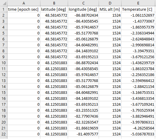
Dynamic Weather Data in the CSV file
The CSV contains time data recorded as seconds from reference epoch in the first column, then three spatial coordinates in the next three columns (degrees latitude and longitude and the altitude above mean sea level, or MSL alt), and finally time-dependent volumetric temperature values in the fifth column.
Reviewing the main function script
Review the code the main function script, vmExampleWeatherCsv2Hdf5.m, to see what the script accomplishes.
- Open vmExampleWeatherCsv2Hdf5.m in MATLAB or a text editor of your choice.
- Examine the code and comments.
- It calls the csv2vmarr helper function to restructure the tabular data in the CSV file into ordered arrays. It reads any CSV file in which data is organized in columns such that the first column represents times in seconds since some reference epoch, the next three columns represent spatial coordinates, and the last column represents some volumetric data. The function produces four ordered arrays (without repeating elements), one for time and three for spatial coordinates, as well as a single four-dimensional array of corresponding volumetric data. In this case, it skips the first row because it contains textual header information. The returned times are in seconds since epoch; latitude, longitude in degrees; altitude in meters; and temperature in degrees Celsius.
- It uses the vmExampleWeatherWriteHdf5 local function to define the header information and to write the volume grid coordinates and volumetric temperature data into a HDF5 file of a specified name. In this case, it creates an Earth-fixed Cartographic grid of four-dimensional temperature data in degrees Celsius.
- The local function calls the createvmgrid helper function to create a blank default structure describing a volumetric grid. It includes a name, parent, type, and description, even if they are blank.
- Finally, the local function calls the writevmhdf5 helper function to write an STK-readable HDF5 file using a specified file name and filled-out structures containing information about the header, times, coordinates, and volumetric data.
- Repeat the process for the three helper function script files to learn more about how they function.
vmExampleWeatherCsv2Hdf5 is an example main function that takes CSV files like DynamicWeatherData.csv, which have flat tables of time-dynamic spatial data, and creates an equivalent HDF5 file (.h5) suitable for loading into the STK application. The script is broken out into sections. Broadly, it does the following:
Calling the main function in MATLAB
Using the example main function vmExampleWeatherCsv2Hdf5, you can accomplish the entire
- Open the MATLAB application.
- Click New on the Editor ribbon to create a new script.
- Set the current MATLAB path to the folder where you've copied the script files and CSV file.
- Copy and paste or enter the following code in the Editor window, replacing
<file path>with the full path to your DynamicWeatherData.csv file. For example,C:\Users\<username>\Documents\STK_ODTK 13\VolumetricWeatherData: - Click Run current section (Ctrl+Enter) on the Editor ribbon.
vmExampleWeatherCsv2Hdf5('<file path>\DynamicWeatherData.csv','my_volumetricExampleScenarioDynamicWeatherData.vmc.h5')
This will create an HDF5 file named my_volumetricExampleScenarioDynamicWeatherData.vmc.
Loading the HDF5 file
Now that you have created your HDF5 file with your weather and volumetric object data, import it into the Volumetric object on the
- Return to the STK application.
- Open VolumetricWeather's () Properties ().
- Select the Basic - Definition page when the Properties Browser opens.
- Select the Load Grid and Computed Data option.
- Click the File ellipsis (
 ).
). - Browse to the location of your my_volumetricExampleScenarioDynamicWeatherData.vmc.h5 file when the Select File dialog box opens.
- Select my_volumetricExampleScenarioDynamicWeatherData.vmc.h5.
- Click to confirm your selection and to close the Select File dialog box.
- Note the changes.
- Click to accept your changes and to keep the Properties Browser open.
The Computed Analysis interval has automatically been set to use the interval defined in the file. Note the number of defined altitude values and number of grid points that make up the grid in the read-only Volume Grid field.
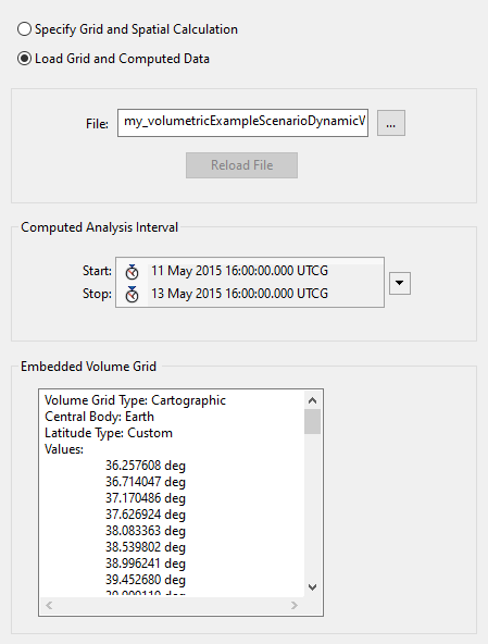
Volumetric basic definition
Updating the dynamic visuals of weather data
Update the graphical properties of the Volumetric object to properly display your data.
Updating the 3D Graphics volumetric attributes
Use the
- Select the 3D Graphics - Attributes page.
- Select the Smoothing check box.
- Select the Shading check box.
- Ensure that Quality is set to High.
Smoothing smooths out the volume and surface boundaries using interpolation between grid points.
Shading adds shading to the boundary surface and generates helpful lighting effects based on surfaces.
A higher quality slows down the animation but reduces the fuzziness of boundaries and increases the density of filled colors.
Updating the 3D Graphics volumetric grid properties
The
- Select the 3D Graphics - Grid page.
- Clear the Show Grid check box.
The Volumetric grid is a collection of enumerated points placed in 3D space using steps taken in each coordinate using various coordinate types. This clears the data for all points based on evaluation over the entire grid.
Updating the 3D Graphics volumetric volume properties
The
- Select the 3D Graphics - Volume page.
- Select the Spatial Calculation Levels option.
- Clear the Immediately update graphics check box.
- In the Show Fill Levels frame, select degC from the Value drop-down menu.
- Click .
Changes are immediately reflected in the 3D graphics window if Immediately update graphics is selected.
The Show Fill Levels option shows color-coded volumes based on how scalar data on grid points fits within multiple threshold levels. Each fill occupies volume where values fall between its specified level and the level immediately above it.
Colorizing the display
Set the color display for the temperate data in the HDF5 file.
- In the Show Fill Levels frame, click .
- Enter the following values:
- Under Ramp Colors, change the Start color to Blue and the Stop color to Red.
- Click .
- Inside the Fill Levels frame, you should see eight evenly spaced values with their correspondingly graded colors. Under the % column, which denotes each value’s translucency level, change the values to the ones shown below:
- Click .
| Option | Value |
|---|---|
| Start Value | -18.15 |
| Stop Value | 16.85 |
| Step Size | 5 |
| Value (C) | Translucency % |
|---|---|
| -18.15 | 10 |
| -13.15 | 25 |
| -8.15 | 60 |
| -3.15 | 57 |
| 1.85 | 55 |
| 6.85 | 35 |
| 11.85 | 35 |
| 16.85 | 48 |
Updating the volumetric 3D Graphics legend
The
- Go to the 3D Graphics - Legends page.
- Select the Show Legend check box.
- In the Text Options panel, change the Title to Temperature (C).
- Click .
Viewing the Volumetric object in the 3D Graphics window
View the visualized weather data, displayed very effectively in expressive colors.
- Bring the 3D Graphics window to the front.
- Right-click on VolumetricWeather () in the Object Browser.
- Select Zoom To in the shortcut menu.
- Click Orient from North (
 ) on the 3D Graphics window toolbar.
 - Click Orient from Top (
 ) on the 3D Graphics window toolbar.
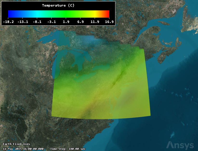
Weather data visualized as a 3D Volumetric object
Animating your dynamic data
With your data finally loaded into a Volumetric object in the STK application, and the graphics now properly configured for display, you can animate your scenario to exhibit the data as it changes over time.
Updating the animation properties
The scenario animation properties control the animation cycle, animation step definition, and the intervals between the refresh updates in the 2D and 3D Graphics windows.
- Open VolumetricWeatherData's () Properties ().
- Select the Basic - Time page.
- Select the Stop at Time check box in the Animation panel.
- Select the Loop at Time animation cycle option from the Stop at Time drop-down list.
- Click .
This will allow the weather data to animate on a loop back from the Start Time so you have time to view the data in motion from different angles.
View the dynamic data in motion
Animate the scenario to view the dynamic weather data.
- Click Increase Time Step (
 ) in the Animation toolbar and set the time step to 180.00 sec.
 - Click Start (
 ) to animate your scenario.
 - Move the camera around so that it looks at the southern edge of the volume in cross-section
- Use your mouse to zoom in on a portion of the volume near the earth's surface.
- When finished, click Reset (
 ) on the Animation Toolbar.
You can see how data display changes over time. The graphics of the Volumetric object convey the changing temperature patterns as they move across the continent.
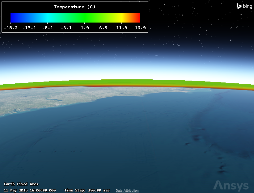
Volumetric cross section
Notice the pronounced temperature difference between altitudes of the volume.
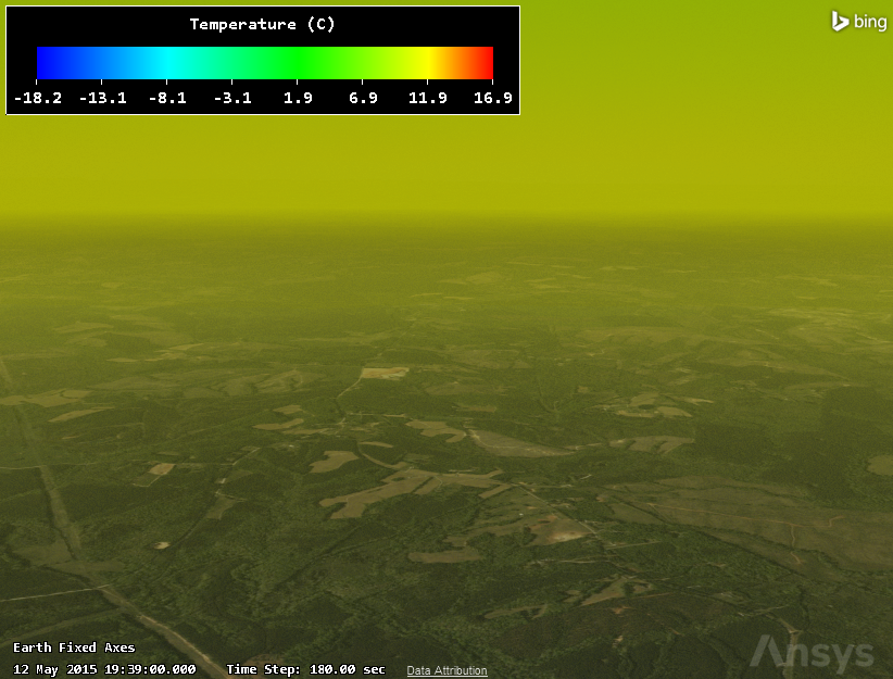
Surface temperature
Notice the temperature difference at the surface compared to higher altitudes.
Saving your work
Close out your scenario and save york work.
- Close any report or tools that are still open.
- Save () your work.
Summary
In this lesson you learned how to take weather data from a CSV file and convert it to the HDF5 format to be used within the STK application. You also created a new scenario and modeled a Volumetric object. Utilizing the example MATLAB scripts, you learned how the data needed to be formatted and what steps the scripts took to convert the file. The final converted file was loaded into the Volumetric object. Next, you modified the 3D Graphics properties to display the temperature data. Finally, you animated the scenario to see the colorized display and how the temperature changed over time.
On your own
There are several demonstrative and explanatory graphical attributes you can change for Volumetric objects, including the Grid, different Volume Boundary and Fill Level gradient scales, and Cross Sections. Explore some of these properties to better understand their uses