State and Configuration |
A NumericalPropagatorDefinition holds collections of PropagationStateElements, AuxiliaryStateElements, and PropagationStateCorrectors, as well as a NumericalIntegrator. The propagation elements represent quantities, such as position, for which no trajectory is known and a set of differential equations can be defined to govern how the propagation element changes over time. The numerical integrator uses the differential equations defined on the propagation elements to advance from one time to the next. In the process, auxiliary values are computed either in the process of integrating the propagation elements or separate from them. However, unlike the propagation elements, the auxiliary elements do not have differential equations to integrate. Lastly, the correctors operate on the propagated elements after each integration step in order to update the values based on discrete criteria above and beyond the differential equations. Altogether, a NumericalPropagatorDefinition uses these collections and integrator in order to create a NumericalPropagator.
The following diagram illustrates the workflow involved in configuring several state elements together to define their relationships to each other. "CustomThrust" represents a model created by a user which can couple the differential equations between the mass and the position (forces).
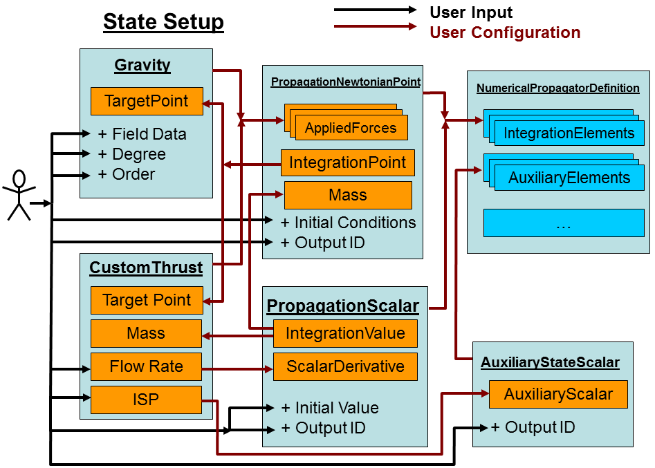
Geometry types such as Scalar, Vector, Point and Axes are used to define the abstract time-varying behavior of elements and dependencies within the state. For instance, the mass is represented by a Scalar which can be either a constant number, an abstract time-varying quantity, or a value representing the current value in the state during integration ("IntegrationMass"). This allows the system to remain agnostic as to whether a given dependency is a constant value, a predefined function of time and other quantities, or an active member of the state, respectively.
In the above example, a user is setting up a problem involving a gravity model and a custom thrust model. The gravity model requires a position ("TargetPoint") and data on the gravitational field to compute in order to produce a specific force. The custom thrust model also depends on the position as well as the current mass and defines a flow rate for the propellant (mass) in addition to being a force model. So, the user adds both force models to define the derivative of the state element for position and then adds the flow rate to define the derivative for the mass. Since the position also needs the mass to determine the acceleration as a result of Newton's Second Law, it gets coupled with the "IntegrationMass" from the state element representing the mass. This way, coupling complex relationships becomes a matter of connecting the geometries (and scalars) together prior to propagation.
This also allows a lot of places for users to customize behavior. If users wish to provide custom time-varying functions for drag coefficients, solar reflectivity coefficients, mass, pointing vectors, or any other elements which depend on geometry, so long as the configuration doesn't use the "integrated" geometry objects (e.g. "IntegrationPoint" or "IntegrationMass") outside of propagation everything will work properly in the propagator. In order to use "integrated" objects outside of propagation, users need to create new geometry objects which define the geometric values based on the time history of the state along with an appropriate interpolation scheme.
After creating a NumericalPropagator from a state, the abstract time-varying geometry is set in the propagator and any changes to the geometry will not impact the results of propagation. To change the results, a new propagator needs to be created after changing the configuration as necessary. If the only change needed is to respecify the initial conditions of the state or the initial epoch, the propagator can be reset to new initial conditions, using the same state and derivatives (force models).
The following example demonstrates this in code:
PropagationScalar mass = new PropagationScalar();
mass.setIdentification("MyVehicleMass"); // Needed to identify output after propagation
mass.setScalarDerivative(massFlowRate);
// To specify a second-order differential equation for mass,
// include a "FirstDerivative" in the Motion for the InitialState.
// Then, the "ScalarDerivative" represents the derivative of the
// mass flow rate.  As a result, both mass and mass flow
// will be integrated by the propagator.
mass.setInitialState(new Motion1<Double>(initialMass));

PropagationNewtonianPoint position = new PropagationNewtonianPoint();
position.setIdentification("MyVehiclePosition"); // Needed to identify output after propagation
position.setInitialPosition(initialPosition);
position.setInitialVelocity(initialVelocity);
position.setIntegrationFrame(earth.getInertialFrame());
position.setMass(mass.getIntegrationValue());

SphericalHarmonicGravity gravity = new SphericalHarmonicGravity();
gravity.setTargetPoint(position.getIntegrationPoint()); // Will represent the position during propagation
SphericalHarmonicGravityModel gravityModel = SphericalHarmonicGravityModel.readFrom(gravityFilePath);
int degree = 41;
int order = 41;
boolean includeTwoBodyForce = true;
SolidTideModel tideModel = null;
gravity.setGravityField(new SphericalHarmonicGravityField(gravityModel, degree, order, includeTwoBodyForce, tideModel));

AtmosphericDragForce drag = new AtmosphericDragForce();
double solarFlux = 150.0;
double kp = 3.00;
ScalarDensityJacchiaRoberts density = new ScalarDensityJacchiaRoberts();
density.setSolarGeophysicalData(new ConstantSolarGeophysicalData(solarFlux, kp));
density.setTargetPoint(position.getIntegrationPoint()); // Will represent the position during propagation
density.setApparentSunPosition(); // More accurate, slightly slower performance
density.setUseApproximateAltitude(true); // Faster, better numerical precision, very slightly worse accuracy
drag.setDensity(density);
drag.setCoefficientOfDrag(Scalar.toScalar(2.2)); // This could be a time varying Scalar instead
drag.setReferenceArea(Scalar.toScalar(20.0));

position.getAppliedForces().add(gravity);
position.getAppliedForces().add(drag);

AuxiliaryStateScalar densityOutput = new AuxiliaryStateScalar(density);
String densityID = "MyAtmosphericDensity";
densityOutput.setIdentification(densityID);

RungeKuttaFehlberg78Integrator integrator = new RungeKuttaFehlberg78Integrator();
integrator.setInitialStepSize(stepSize);

NumericalPropagatorDefinition state = new NumericalPropagatorDefinition();
state.setEpoch(epoch);
state.setIntegrator(integrator);
state.getIntegrationElements().add(position);
state.getIntegrationElements().add(mass);
state.getAuxiliaryElements().add(densityOutput);
The most common element to add to the state is a PropagationNewtonianPoint, which is used to represent the position and velocity of an object during propagation. A list of ForceModels and a Scalar mass are used to define the acceleration on the body of interest using Newton's Second Law. The Newtonian position type exists to make composing forces together into equations of motion easier and avoid confusion arising from different reference frames and representations of the forces. This way, the propagator doesn't have to worry about the complexities of Newton's Law requiring its equations of motion to be integrated in an inertial ReferenceFrame.
In addition to PropagationNewtonianPoint, PropagationScalar and PropagationVector are available to represent any arbitrary scalar or vector quantities and their derivatives. For instance, the scalar state element could represent an angle of attack, a dynamic coefficient of drag, or a collection of scalar state elements could represent any arbitrary user data set. The only restriction is that the user needs to define the set of differential equations by providing the derivatives of the highest order derivative (or value) represented in each state element. The only real distinction between a PropagationNewtonianPoint and a PropagationVector is that the PropagationNewtonianPoint is more explicit in how it defines its derivative (acceleration) and automatically resolves the different forces into a common frame. In contrast, a PropagationVector requires the user to handle all of the frame information when defining the derivative.
Unlike PropagationStateElements, AuxiliaryStateElements are not determined by integration but are instead evaluated directly during the process of propagation. These are things like atmospheric density, percentage illumination, values of forces, and any other scalar or vector values that the user wants to compute and store in the resulting ephemeris. In some cases, it is more efficient to take advantage of the evaluations performed during propagation to avoid redundant computation as well as providing a means of keeping track of intermediate values used in propagating state elements.
PropagationStateCorrectors are used for any modifications to the propagation state that should occur in between integration time steps. This includes any calculations to correct for discontinuities during propagation, such as solar boundary mitigation, or to model any small impulsive forces that occur during propagation. Correctors are completely optional and are not required in order to create a propagator.