Covariance and Uncertainty

In addition to propagating the state elements forward in time, a NumericalPropagator can be used to calculate the values of the state covariance over time. The state covariance describes the uncertainty of the state elements and is not directly propagated. Instead, a StateTransitionMatrix is added to NumericalPropagatorDefinition.IntegrationElements (get) prior to creating the NumericalPropagator. The propagated StateTransitionMatrix data can then be used to find the state covariance at each time step.

StateTransitionMatrix

The state transition matrix represents the transformation from the state at one time to the state at another time. This can be used as an alternative to propagating a state in time with NumericalPropagator, but is more often used in order to find the time-varying covariance of the state. This is because the construction of a StateTransitionMatrix whose equations of motion are a linearization of the equations of motion for the state, and in most cases calculating the derivatives of the state transition matrix takes as long or longer as calculating the derivatives of the state. The NumericalPropagator integrates the state transition matrix completely in parallel to the other integration elements. In addition, the overhead from propagating both the state transition matrix and other state elements simultaneously is minimal due to the redundant calculations. See the Evaluators And Evaluator Groups topic for more information on this optimization.

The StateTransitionMatrix is actually an expanded state transition matrix, also known as a complete consider covariance matrix. In addition to adding state elements to the StateTransitionMatrix you can also add consider parameters. For example, if you wanted to model uncertainty in the drag force in your covariance, you could add the coefficient of drag, or the reference area, as a consider parameter. If no consider parameters are added, the StateTransitionMatrix is identical to a typical state transition matrix. If consider parameters are added, then the StateTransitionMatrix takes the following form:

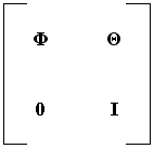
If the cumulative dimension of the state elements is N, and the cumulative dimension of the consider parameters is M, then Φ is an ordinary state transition matrix: an NxN matrix equal to the partials of the state at time t_j with respect to the state at time t_i. Θ is an NxM matrix equal to the partials of the state at time t_j with respect to the consider parameters at time t_i, and the zero and identity matrices are size MxN and MxM, respectively. The complete consider covariance matrix is a square matrix with a dimension of N+M.

Setting Up a StateTransitionMatrix

The derivative of a StateTransitionMatrix is calculated using the IPartialDifferentiable and PartialDerivativesEvaluator types. State elements and derivatives which implement the IPartialDifferentiable interface can be added to the StateTransitionMatrix. The partial derivatives of these types are used to calculate the derivative of the state transition matrix and propagate it forward in time.

In creating the derivative evaluator, the dependencies of the state elements also calculate their partial derivatives, so they too must implement IPartialDifferentiable. All of the included ForceModels have partial derivatives, as do many geometry types in DME Component Libraries, such as ScalarFixed, ScalarSum, ScalarProduct, and ScalarExponent. However, if propagating with additional types, such as user-defined forces, those types will have to implement IPartialDifferentiable as well, or else an exception will be thrown.

To add a variable as a state parameter to the StateTransitionMatrix, call the addStateParameter method, providing the state parameter along with its derivative. When calculating partial derivatives, the derivatives of a value are seen as entirely separate and independent entities. For example, a force could have non-zero partial derivatives with respect to position, with zero partial derivatives with respect to velocity, or vice-versa.

To obtain a higher order representation of a geometry type, call the appropriate method to create a instance that represents the derivative:

Point also has createVectorVelocity and createVectorAcceleration methods for convenience.

These derivative creation methods are virtual methods on the Point, Vector, and Scalar base classes. The default implementations do not produce types which implement IPartialDifferentiable, however, derived classes which themselves implement IPartialDifferentiable (such as the PointPropagationParameter stored as PropagationNewtonianPoint.IntegrationPoint (get)) do create derivatives which implement IPartialDifferentiable. When defining your own geometry type for use with partial derivatives, the base class methods to create derivatives must be overridden to produce an instance with the proper partial derivatives for your custom type.

As a last note, when taking partial derivatives of an object being propagated, the PropagationStateElement is the definitional object responsible for the partial derivatives of the order of the object that is acting as a derivative for the NumericalPropagator. So, a PropagationNewtonianPoint is the definitional object that produces a partial derivatives evaluator for the acceleration of the corresponding position.

Adding a consider parameter is a similar process which is done via the StateTransitionMatrix.addConsiderParameter method. Unlike a state parameter, no derivative is required.

Here is an example where the position and velocity of the point represented by a PropagationNewtonianPoint are added to a StateTransitionMatrix as state parameters. The coefficient of drag is then added as a consider parameter.

Java

Copy

// propagationPoint is a previously initialized PropagationNewtonianPoint.
// drag is a previously initialized AtmosphericDragForce.
StateTransitionMatrix stateMatrix = new StateTransitionMatrix();

IPartialDifferentiable position =
    (IPartialDifferentiable) propagationPoint.getIntegrationPoint();
IPartialDifferentiable velocity =
    (IPartialDifferentiable) propagationPoint.getIntegrationPoint().createVectorVelocity(propagationPoint.getIntegrationFrame());

stateMatrix.addStateParameter(position, velocity);
stateMatrix.addStateParameter(velocity, propagationPoint);
stateMatrix.addConsiderParameter((IPartialDifferentiable) drag.getCoefficientOfDrag());

Raw State to Useful Output

The state at t_j can be found by premultiplying the state vector at t_i by the (t_i -> t_j) state transition matrix. Similarly, the covariance matrix at time t_j can be found by pre and post-multiplying the covariance matrix at t_i by the (t_i -> t_j) state transition matrix. So, by propagating the state transition matrix, the covariance can be found at matching times from an initial covariance, even though the covariance is not itself directly propagated.

The StateTransitionMatrix.populateCovarianceCollection method does this transformation, accepting an initial covariance matrix and a DateMotionCollection1<Matrix>, of state transition matrices and returning a corresponding DateMotionCollection1<Matrix>, of covariance matrices, as seen in the following example:

Java

Copy

// propagator is a previously initialized NumericalPropagator.
// stateMatrix is the StateTransitionMatrix declared and initialized in the last code snippet.
NumericalPropagationStateHistory history = propagator.propagate(propagationTime, 1);
DateMotionCollection1<Matrix> stateTransitionMatrices = history.getDateMotionCollection(stateMatrix.getIdentification());

DateMotionCollection1<Matrix> covarianceMatrices = StateTransitionMatrix.populateCovarianceCollection(initialCovariance, stateTransitionMatrices,
        stateMatrix.getTransitionType());

Covariance Interpolation and Blending

An orbit's position covariance information forms a collection of 3 by 3 matrices that can be interpolated for any orbit type using Covariance3By3SizeAndOrientationInterpolator. The following code snippet shows how to create an interpolator and use it to estimate the position covariance at a time in between the two given times.

Java

Copy

// Position covariance information is interpolated between two covariance matrices
// that are spaced one minute apart.
JulianDate time1 = new GregorianDate(2023, 1, 1).toJulianDate();
JulianDate time2 = time1.addSeconds(60.0);
Matrix3By3 matrix1 = new Matrix3By3(25.0, 0.0, 0.0,
                                    0.0, 36.0, 0.0,
                                    0.0, 0.0, 49.0);
Matrix3By3 matrix2 = new Matrix3By3(2.56032624411e+001, 5.15776932321e-003, 1.08868870033e-002,
                                    5.15776932321e-003, 3.61860979932e+001, 2.16157690194e-004,
                                    1.08868870033e-002, 2.16157690194e-004, 4.91230990929e+001);

// This performs an eigen-decomposition on the matrices that provides the minor, intermediate, and major axis sizes
// (sigmas) and the orientation of the 3D covariance ellipsoid given by the matrices. This information is needed to
// perform the interpolation.
Covariance3By3SizeAndOrientation covariance1 = new Covariance3By3SizeAndOrientation(Matrix3By3Symmetric.fromLowerTriangular(matrix1));
Covariance3By3SizeAndOrientation covariance2 = new Covariance3By3SizeAndOrientation(Matrix3By3Symmetric.fromLowerTriangular(matrix2));
DateMotionCollection2<Covariance3By3SizeAndOrientation, Covariance3By3Derivative> covarianceData =
        new DateMotionCollection2<Covariance3By3SizeAndOrientation, Covariance3By3Derivative>();

covarianceData.add(time1, covariance1);
covarianceData.add(time2, covariance2);

// Lagrange interpolation is used to interpolate the sigmas of the covariance ellipsoid, and Hermite interpolation
// is used to interpolate the orientation.
LagrangePolynomialApproximation interpolationMethod1 = new LagrangePolynomialApproximation();
HermitePolynomialApproximation interpolationMethod2 = new HermitePolynomialApproximation();

// Because there are only two data points, degree 1 interpolation is used.
Covariance3By3SizeAndOrientationInterpolator interpolator = new Covariance3By3SizeAndOrientationInterpolator(interpolationMethod1, 1, interpolationMethod2, 1, covarianceData);
EvaluatorGroup group = new EvaluatorGroup();
Covariance3By3Evaluator evaluator = interpolator.getEvaluator(group);

// Interpolate to estimate the covariance of the spacecraft at the midpoint between the two given times.
Covariance3By3SizeAndOrientation midpointCovariance = evaluator.evaluate(time1.addSeconds(30.0));

// Convert the sigmas and orientation of the interpolated covariance ellipsoid back into matrix form.
Matrix3By3 midpointMatrix = midpointCovariance.toMatrix3By3();

An orbit's position and velocity covariance information forms a collection of 6 by 6 matrices that can be interpolated using blending for orbits that are in orbit regimes that are approximately two-body. (Numerical integration should be used for orbits in three-body orbit regimes.) Covariance6By6TwoBodyBlender is the type used to perform this blending.

The following code snippet illustrates how to use numerical integration to produce dense covariance data that can be compared with data that is produced by blending sparse covariance data.

Java

Copy

// Get Earth from the current central body facet.
EarthCentralBody earth = CentralBodiesFacet.getFromContext().getEarth();

// Set up a numerical propagator that uses two-body gravitational force only.
JulianDate epoch = new JulianDate(new GregorianDate(2023, 1, 1));

Cartesian initialPosition = new Cartesian(6575800.000, 0.000000, 0.000000);
Cartesian initialVelocity = new Cartesian(0.000000, 4317.0, 7477.0);
final double stepSize = 60.0;
final double durationDays = 1.0;
final double totalTime = durationDays * 86400.0;

final double mass = 1000.0;
NumericalPropagatorDefinition state = new NumericalPropagatorDefinition();

// Set up force models and initial conditions.
PropagationNewtonianPoint posAndVel = new PropagationNewtonianPoint("Test", earth.getInternationalCelestialReferenceFrame(), initialPosition, initialVelocity);
posAndVel.setMass(Scalar.toScalar(mass));

state.setEpoch(epoch);
state.getIntegrationElements().add(posAndVel);

TwoBodyGravity gravity = new TwoBodyGravity(posAndVel.getIntegrationPoint());
posAndVel.getAppliedForces().add(gravity);

IPartialDifferentiable position =
        (IPartialDifferentiable) posAndVel.getIntegrationPoint();
IPartialDifferentiable velocity =
        (IPartialDifferentiable) posAndVel.getIntegrationPoint().createVectorVelocity(posAndVel.getIntegrationFrame());

StateTransitionMatrix stateMatrix = new StateTransitionMatrix();
stateMatrix.addStateParameter(position, velocity);
stateMatrix.addStateParameter(velocity, posAndVel);
state.getIntegrationElements().add(stateMatrix);

RungeKuttaFehlberg78Integrator integrator = new RungeKuttaFehlberg78Integrator();
integrator.setRelativeTolerance(1e-15);
integrator.setMinimumStepSize(stepSize);
integrator.setMaximumStepSize(stepSize);
integrator.setInitialStepSize(stepSize);
integrator.setStepTruncationOrder(-3);
integrator.setStepSizeBehavior(KindOfStepSize.FIXED);

state.setIntegrator(integrator);

// Provide an initial covariance matrix that is a diagonal matrix.
DenseMatrix initialCovariance = new DenseMatrix(6, 6);
initialCovariance.set(0, 0, 25.0); // XX position variance, m^2.
initialCovariance.set(1, 1, 25.0); // YY position variance, m^2.
initialCovariance.set(2, 2, 25.0); // ZZ position variance, m^2.
initialCovariance.set(3, 3, 1.0e-4); // VxVx velocity variance, m^2/s^2.
initialCovariance.set(4, 4, 1.0e-4); // VyVy velocity variance, m^2/s^2.
initialCovariance.set(5, 5, 1.0e-4); // VzVz velocity variance, m^2/s^2.

// Propagate to get a dense numerical covariance collection to serve as the truth model.
NumericalPropagator propagator = state.createPropagator();
NumericalPropagationStateHistory numericalHistory = propagator.propagate(Duration.fromSeconds(totalTime), 1);
DateMotionCollection1<Matrix> numericalTransitions = numericalHistory.getDateMotionCollection(stateMatrix.getIdentification());
DateMotionCollection1<Matrix> numericalCovariance = StateTransitionMatrix.populateCovarianceCollection(initialCovariance, numericalTransitions, stateMatrix.getTransitionType());

// Reset the propagator so that a sparse covariance collection can be produced.
propagator.reset();

NumericalPropagationStateHistory sparseHistory = propagator.propagate(Duration.fromSeconds(totalTime), 3);
DateMotionCollection1<Cartesian> sparseStates = sparseHistory.getDateMotionCollection(posAndVel.getIdentification());
DateMotionCollection1<Matrix> sparseTransitions = sparseHistory.getDateMotionCollection(stateMatrix.getIdentification());
DateMotionCollection1<Matrix> sparseCovariance = StateTransitionMatrix.populateCovarianceCollection(initialCovariance, sparseTransitions, stateMatrix.getTransitionType());

// Create a blender using the sparse state collection and covariance collection.
// Both the state and the covariance data are in Earth's inertial ICRF frame.
Covariance6By6TwoBodyBlender blender = new Covariance6By6TwoBodyBlender(sparseStates, sparseCovariance, earth.getInternationalCelestialReferenceFrame(),
        earth.getInternationalCelestialReferenceFrame().getAxes(), earth.getInternationalCelestialReferenceFrame(),
        WorldGeodeticSystem1984.GravitationalParameter);

DynamicMatrixEvaluator evaluator = blender.getEvaluator();

// This blending reproduces the dense numerical covariance collection from the sparse collection to high precision.
DateMotionCollection1<Matrix> blendedCovariance = evaluator.evaluate(epoch, epoch.addDays(1.0), Duration.fromSeconds(60.0), 0);