STK Premium (Air), STK Premium (Space), or STK Enterprise
You can obtain the necessary licenses for this tutorial by contacting AGI Support at support@agi.com or 1-800-924-7244.
Required product install: The Ansys ModelCenter® model-based systems engineering software and the STK Plugin for ModelCenter are required to complete this tutorial.
ModelCenter installation prerequisites: The ModelCenter software requires the installation of a 64-bit version of Java, a 64-bit implementation of Python 3.x, and the installation of the thrift and six Python packages. See the ModelCenter Installation Prerequisites for more information.
This tutorial was written using version 2026 R1 of the Ansys ModelCenter® model-based systems engineering software.
The results of the tutorial may vary depending on the user settings and data enabled (online operations, terrain server, dynamic Earth data, etc.). It is acceptable to have different results.
Capabilities covered
This lesson covers the following capabilities of the Ansys Systems Tool Kit® (STK®) digital mission engineering software:
- STK Pro
- Coverage
- Communications
- STK Analyzer
- STK Analyzer Optimization
Problem statement
Engineers and operators want to analyze the design of an onboard communications system for a satellite in geosynchronous orbit (GEO). Specifically, they need to better understand the requirements for the satellite's transmitter, which must link to facilities spanning the contiguous United States (CONUS). You want to study the transmitter's design parameters in order to provide the optimal link closure across CONUS, measured in terms of a high ratio of energy per bit to noise spectral density (Eb/No).
Solution
Use the STK software's Coverage and Communications capabilities and Analyzer capability, which is part of the Ansys ModelCenter® model-based systems engineering software, to run a series of trade studies so that you can better understand how the satellite transmitter's configuration affects its coverage capability. Then, use the STK Analyzer Optimization capability to optimize your satellite transmitter's parameters.
What you will learn
Upon completion of this tutorial, you will be able to:
- Analyze a communication system for trends
- Optimize communications parameters to meet mission objectives
- Perform Parametric, Carpet Plot, and Optimization studies that vary input variables through a range of values
Using the starter scenario
To speed things up and allow you to focus on the portion of this exercise that teaches you how to use the ModelCenter software, a partially created scenario has been provided for you.
Opening the starter scenario
The starter scenario is included in your install.
- Launch the STK application (
 ).
). - Click
 Open a Scenario in the Welcome to STK dialog box.
 - Browse to <Install Dir>\Data\Resources\stktraining\VDFs.
- Select Analyzer_Comm_Analysis.vdf.
- Click .
Saving the VDF as a scenario file
Save and extract the VDF data in the form of a scenario folder. When you save a VDF in the STK application, it will save in its originating format. That is, if you open a VDF, the default save format will be a VDF (.vdf). If you want to save and extract a VDF as a scenario folder, you must change the file format by using the Save As feature. This will create a permanent scenario file complete with child objects and any additional files packaged with the VDF.
- Open the File menu when the starter scenario opens.
- Select Save As....
- Select the STK User folder in the navigation pane when the Save As dialog box opens.
- Select the Analyzer_Comm_Analysis folder.
- Click .
- Select Scenario Files (*.sc) in the Save as type drop-down list.
- Select the Analyzer_Comm_Analysis scenario file in the file browser.
- Click .
- Click in the Confirm Save As Dialog box to overwrite the existing scenario file in the folder and to save your scenario.
A scenario folder with the same name as the VDF was created for you when you opened the VDF in the STK application. This folder contains the temporarily unpacked files from the VDF.
When saving a VDF as a scenario folder, you should extract its contents to the scenario folder the STK application automatically creates for you in the STK User folder. See the
Save (![]() ) often during this lesson!
) often during this lesson!
Reviewing the starter scenario
In the 2D Graphics window, Geo_Sat's sensor, Tgt_Centroid, is boresighted at the geographic center of the contiguous United States, represented by a Place object, Centroid. A Transmitter object, DL_Tx, is attached to Geo_Sat's sensor. DL_Tx is using a
- Right-click on EbNo_Avg (
 ) in the Object Browser.
 - Select Report & Graph Manager... (
 ) in the shortcut menu.
 - Select the Grid Stats (
 ) report in the Installed Styles (
 ) folder.
 - Click .
- Review the Grid Stats report.
- Close the report and the Report & Graph Manager.
- Save (
 ) your scenario.
 - Close the STK application.
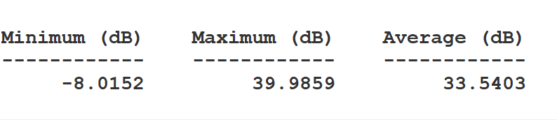
Grid Stats Report
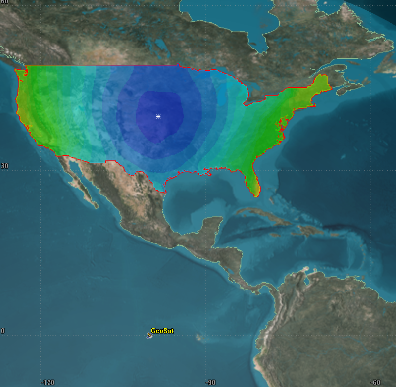
The contours of the Figure of Merit are based on the minimum and maximum values in the report. You will notice some areas of CONUS do not have particularly good access to Geo_Sat with the given configuration of Geo_Sat's transmitter.
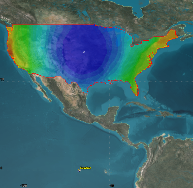
UnOptimized Coverage over CONUS
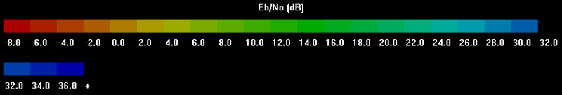
You can enable the legend on the Figure of Merit - 2D Graphics - Static page.
Creating a new ModelCenter project
The
- Open the ModelCenter (
 ) application.
 - Click in the Welcome to ModelCenter dialog box.
- Click when the What type of model would you like to create? dialog box opens.
- Navigate to your scenario folder (for example, C:\Users\<username>\Documents\STK_ODTK 13\Analyzer_Comm_Analysis.
- Enter Analyzer_Comm_Analysis in the File name field.
- Ensure the Save as type is set to the ModelCenter Model (Zip) (*.pxcz).
- Click .
Launching the STK Plugin for ModelCenter
The
- Select favorites (
 ) in the Server Browser at the bottom of the window.
 - Click and drag the STK component (
 ) into the dashed circle underneath "Drop items here to build the model" in the workflow's Analysis View.
 - Select Analyzer_Comm_Analysis.sc when the Open STK Scenario file dialog box opens.
- Click .
- After a few moments, the STK Analyzer window will open.
The Analyzer_Comm_Analysis scenario file will open in the STK application in the background.
You can add any of the STK variables as ModelCenter input or output variables through the STK Analyzer window that appears. If you change the value of a variable in your scenario through the STK interface or the ModelCenter Component Tree, you should re-add the variable into ModelCenter or re-run the workflow before running any trade studies with the new value.
Setting up your analysis with Analyzer
Your goal for this problem is to optimally configure the satellite's transmitter to best provide link closure to all facilities via a high Eb/No. These studies will focus on Eb/No, but there are a handful of parameters that will impact your study, including:
- Power
- Frequency
- Data Rate
- Antenna diameter
Use the STK Analyzer window to configure the input and output variables available for further analysis with the
Selecting the transmitter model specs input variables
Your studies will focus on several design specifications of the satellite's transmitter. Before you can use them in your model, however, you must first add them to your design space.
- Select GeoSat (
 ) in the STK Variables tree.
 - Note that GeoSat has automatically been expanded to show Tgt_Centroid (
 ).
). - Expand (
 ) Tgt_Centroid ().
 - Select DL_Tx (
 ).
). - In the STK Property Variables tree, expand () Model (Complex_Transmitter_Model) (
 ).
). - Expand () ModelSpecs ().
- Select Power (
 ).
). - Move (
 ) Power () to the Analyzer Variables list.
 - Select Frequency ().
- Move () Frequency () to the Analyzer Variables list as an input variable.
When you select an object in the STK Variables tree, all possible input variable candidates for that object are listed under the General tab and the Active Constraints tab in the STK Property Variables panel.
Note that both Power and Frequency are listed under Inputs in the Analyzer variables list.
Selecting the transmitter modulator data rate as an input variable
In addition to the transmitter model specs, you want to study the impact of the data rate from the transmitter's modulator.
- Expand () Modulator ().
- Move () DataRate () to the Analyzer Variables list as another input variable.
Selecting the antenna diameter as an input variable
While the satellite's antenna diameter is fixed at 1 meter in this scenario, it is helpful to study it in order to understand how the antenna's diameter affects Eb/No.
- Expand () the Antenna () property.
- Expand () the ModelSpec () property.
- Select Diameter ().
- Move () Diameter () to the Analyzer Variables list as an input variable.
Note that Diameter has been added under Inputs in the Analyzer variables list.
Adding the output variables
The same data providers that are available in the Report & Graph Manager in the STK application are available in the Data Provider Variables tree.
- In the STK Variables tree, expand () CONUS_Cov (
 ).
). - Select EbNo_Avg ().
- In the Data Provider Variables tree, expand () the Overall Value (
 ) data provider.
 - Move () the following data provider elements (
 ) into the Analyzer Variables list:
 - Minimum
- Maximum
- Average
- Click to confirm your selections and to close the STK Analyzer window.
Note that the variables are listed as Outputs in the Analyzer Variables list.
This will also close the STK application, which had been running in the background.
Determining the impact of power on coverage
The first study you will perform varies the transmitter's power to determine which value is best.
Using the Parametric Study tool
The Parametric Study tool runs a workflow through a sweep of values for some input variable. You can plot the resulting data to view trends.
- Expand (
 ) all the elements in the Component Tree.
 - Click Parametric Study (
 ) in the Standard toolbar.
 - Click and drag Power (
 ) from the Component Tree to the Design Variable field when the Parametric Study tool opens.
 - Set the following Design Variable values:
- Click and drag Minimum (
 ), Maximum (), and Average () from the Component Tree to the Responses field.
 - Click .
| Option | Value |
|---|---|
| starting value | 300 |
| ending value | 3000 |
| number of samples | 10 |
Note that the step size is automatically set to 300.
Clicking will open the Data Explorer, which is a tool used by Trade Study tools to display data while they are being collected from your Model. While data are being collected, the Data Explorer displays a progress meter, a halt button, and the data. The Table page of the Data Explorer displays trade study data in a tabular form. It is the default window that is present for all trade studies. Cells are shaded differently depending on the associated variable's state. Input variables are shown with green text, valid values are displayed with black text, invalid values are displayed with gray text, and modified values are displayed with blue text. From the table it is possible to view and edit all values in your trade study and even to add and remove whole runs.
Creating a 2D Line Plot
Once the trade study is complete and all data have been collected, the Data Explorer toolbar becomes active. The Data Explorer stores values for all variables in a workflow and special variables from the trade study. Some trade study tools will automatically launch a default plot window when the trade study runs. For other plots, you can create them from the Add View menu. For this study, you will create a 2D Line Plot. A 2D Line Plot displays an X-Y plot for variables in your model. Any variable in the workflow can be plotted against any other variable.
- Close the 2D Scatter Plot that opened when the trade study finished running.
- Click Add View (
 ) on the Table Page toolbar.
 - Select 2D Line Plot (
 ) in the drop-down menu.
Setting the plot variables
The chart shows Minimum versus Power. You could change the y dimension to Maximum or Average to adjust the plot as needed. However, you will add Maximum and Average to the plot results for comparison on one plot. Use the Plot Options menu to set which variable is displayed on which axis. In certain plots, you can set other global plot controls based on the plot variables. In this case, you want to view several variables: the minimum, maximum, and average power.
- Click Dimensions in the Plot Options menu on the left-hand side of the 2D Line Plot.
- Click Add Series (+).
- Set Series 2 - x to Power.
- Set Series 2 - y to Maximum.
- Click Add Series (+).
- Set Series 3 - x to Power.
- Set Series 3 - y to Average.
- Click on the plot to close the Plot Options menu.
This adds the Maximum power values to the plot.
This adds the Average power values to the plot.
Setting options for the axes
Use the Axes tab to set options for the axes.
- Click Axes in the Plot Options menu.
- Select the Ticks tab.
- Change the Max # value to 40.
- Click anywhere on the plot to close the Plot Options menu.
- Review the 2D Line Plot.
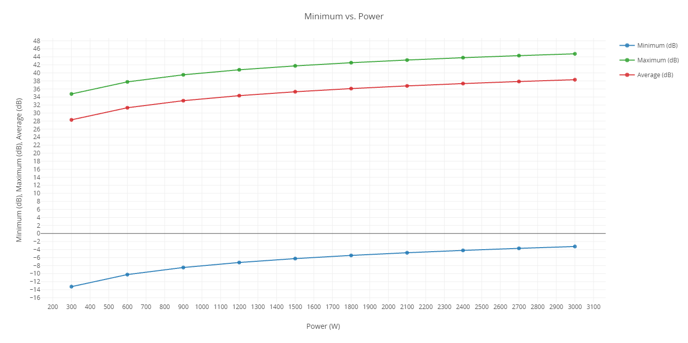
Eb/No Vs. Power 2D Line Plot
Recall that this trade study is designed to help give you an understanding of which power setting to use for the transmitter to give the best overall minimum Eb/No. Your focus is on Power versus Minimum at 0 dB. Note that the minimum dB does not approach 0 for the given values. You have a greater range of power in watts with which you can work in your design.
Closing out your trade study
Close out your trade study for the next section.
- Close the 2D Line Plot and the Table page when you are finished.
- Click when prompted to close your trade study without saving.
- Leave the Parametric Study tool open.
Rerunning with adjusted values
Adjust the Power Design Variable values by a factor of 10.
- Increase the Power Design Variables by setting the following values:
- Click .
- Close the 2D Scatter Plot that automatically opened after the trade study finished running.
- Click Add View () on the Table Page toolbar.
- Select 2D Line Plot () in the drop-down menu.
- Click Axes in the Plot Options menu.
- Select the Ticks tab.
- Change the Max # value to 40.
- Click on the plot to close the Plot Options menu.
- Review the 2D Line Plot.
| Option | Value |
|---|---|
| starting value | 3000 |
| ending value | 30000 |
| number of samples | 10 |
| step size | 3000 |
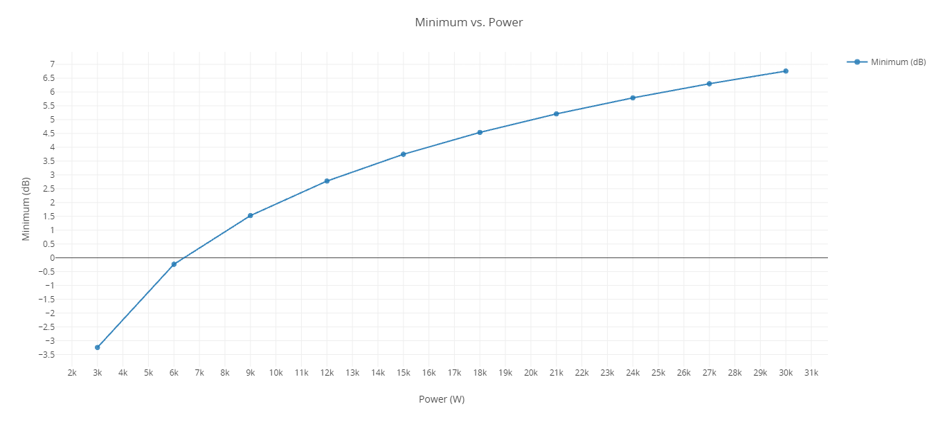
Minimum Eb/No Vs. power 2D Line Plot
Looking at the 2D Line Plot, you can see that Power versus Minimum at 0 dB is reached with a power level somewhere between 6,000 and 7,000 watts.
Closing out your trade study
Close out your trade study for the next section.
- Close the 2D Line Plot and the Table page when you are finished.
- Click when prompted to close your trade study without saving.
- Leave the Parametric Study tool open.
Determining the impact of frequency on coverage
Power is not the only transmitter parameter that will impact your coverage. Frequency also has an impact. To determine how much, run another Parametric Study.
Running a Parametric Study
Build a new Parametric Study using Frequency as your Design Variable.
- Click and drag Frequency () from the Component Tree to the Design Variable field when the Parametric Study tool opens.
- Set the following Design Variable values:
- Click .
- Close the 2D Scatter Plot that automatically opened after the trade study finished running.
- Click Add View () on the Table Page toolbar.
- Select 2D Line Plot () in the drop-down menu.
This will replace Power as the Design Variable.
| Option | Value |
|---|---|
| starting value | 10 |
| ending value | 20 |
| number of samples | 11 |
Updating the 2D Line Plot's variables
The chart shows Minimum versus Frequency. Add the Maximum and Average variables to the plots results for comparison on one plot.
- Click Dimensions in the Plot Options menu on the left-hand side of the 2D Line Plot.
- Click Add Series (+).
- Set Series 2 - x to Frequency.
- Set Series 2 - y to Maximum.
- Click Add Series (+).
- Set Series 3 - x to Frequency.
- Set Series 3 - y to Average.
- Click on the plot to close the Plot Options menu.
- Review the 2D Line Plot.
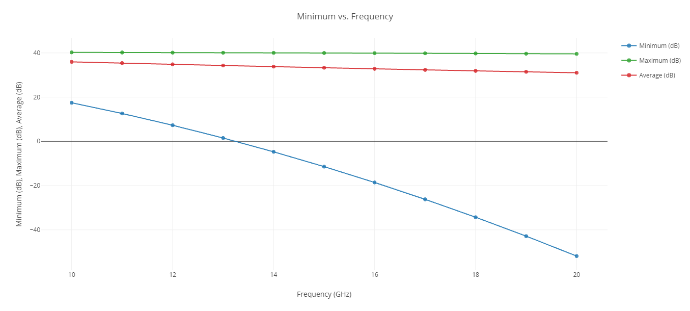
Eb/No Vs. Frequency 2D Line Plot
Eb/No decreases with frequency due to an increase in propagation loss and decrease in Gaussian Antenna gain, where Gaussian is the default antenna type you are using on the transmitter. You can see that frequencies less than 13 GHz will assure you of an Eb/No greater than 0 for all of CONUS.
Closing out your trade study
Close out your trade study for the next section.
- Close the 2D Line Plot and the Table page when you are finished.
- Click when prompted to close your trade study without saving.
- Leave the Parametric Study tool open.
Determining the impact of data rate on coverage
The next parameter impacting coverage is the data rate of the transmitter. For this study, you will vary the data rate from 10 to 20 Mb/sec (megabits per second).
Running the Parametric Study
With DataRate added as an input variable, build your Parametric Study.
- Click and drag DataRate () from the Component Tree to the Design Variable field when the Parametric Study tool opens.
- Set the following Design Variable values:
- Click .
- Close the 2D Scatter Plot that automatically opened after the trade study finished running.
- Click Add View () on the Table Page toolbar.
- Select 2D Line Plot () in the drop-down menu.
This will replace Frequency as the Design Variable.
| Option | Value |
|---|---|
| starting value | 10e+06 |
| ending value | 20e+06 |
| number of samples | 11 |
Updating the 2D Line Plot's variables
The chart shows Minimum versus DataRate. Add the Maximum and Average variables to the plots results for comparison on one plot.
- Click Dimensions in the Plot Options menu on the left-hand side of the 2D Line Plot.
- Click Add Series (+).
- Set Series 2 - x to DataRate.
- Set Series 2 - y to Maximum.
- Click Add Series (+).
- Set Series 3 - x to DataRate.
- Set Series 3 - y to Average.
- Click on the plot to close the Plot Options menu.
- Review the 2D Line Plot.
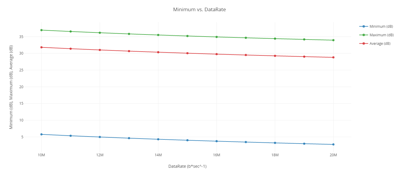
Eb/No Vs. Data Rate 2D Line Plot
Note that coverage decreases with increased data rate. Decreasing the data rate equivalently decreases the bandwidth and increases the Eb/No.
Closing out your trade study
Close out your trade study for the next section.
- Close the 2D Line Plot and the Table page when you are finished.
- Click when prompted to close your trade study without saving.
- Leave the Parametric Study tool open.
Determining the impact of antenna diameter on coverage
The next parameter you will examine is the diameter of the antenna for the transmitter. Although this isn't part of the transmitter's optimization, it's an interesting study. For this study, you will vary the size of the diameter from 0.5 to 2 meters.
Running the Parametric Study
Build your Parametric Study using Diameter as the Design Variable.
- Click and drag Diameter () from the Component Tree to the Design Variable field when the Parametric Study tool opens.
- Set the following Design Variable values:
- Click .
- Close the 2D Scatter Plot that automatically opened after the trade study finished running.
- Click Add View () on the Table Page toolbar.
- Select 2D Line Plot () in the drop-down menu.
This will replace DataRate as the Design Variable.
| Option | Value |
|---|---|
| starting value | 0.5 |
| ending value | 2 |
| number of samples | 16 |
Updating the 2D Line Plot's variables
The chart shows Minimum versus Diameter. Add the Maximum and Average variables to the plots results for comparison on one plot.
- Click Dimensions in the Plot Options menu on the left-hand side of the 2D Line Plot.
- Click Add Series (+).
- Set Series 2 - x to Diameter.
- Set Series 2 - y to Maximum.
- Click Add Series (+).
- Set Series 3 - x to Diameter.
- Set Series 3 - y to Average.
- Click on the plot to close the Plot Options menu.
- Review the 2D Line Plot.
- Close the 2D Line Plot when you are finished.

Eb/No Vs. Diameter 2D Line Plot
Notice that while the maximum and for the most part average Eb/No values rise with increasing antenna size, the minimum value decreases. The maximum coverage value increases with increasing antenna diameter, however you do see diminishing returns. The reason for this is that as antenna size increases, the gain increases while the beamwidth decreases.
Looking closer at the average
Locations farthest from the antenna boresight see their Eb/No values drop as the beamwidth decreases. Take a closer look at the average coverage.
- Return to the Table page.
- Click Add View () on the Table Page toolbar.
- Select 2D Line Plot () in the drop-down menu.
- Click Dimensions in the Plot Options menu on the left-hand side of the 2D Line Plot.
- Set the y axis to Average.
- Click Axes in the Plot Options menu.
- Select the Ticks tab.
- Change Max # to 20.
- Click on the plot to close the Plot Options menu.
- Review the 2D Line Plot.
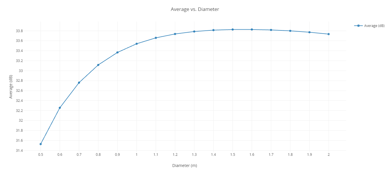
Average Eb/No Vs. Antenna Diameter 2D Line Plot
The average Eb/No value reaches a peak value at an antenna diameter of about 1.5 m (meters) and then the average Eb/No values begin to decrease.
Closing out your trade study
Close out your trade study for the next section.
- Close the 2D Line Plot and the Table page when you are finished.
- Click when prompted to close your trade study without saving.
- Close the Parametric Study tool.
Determining if power and frequency impact one another
You have determined that power and frequency have significant impacts on coverage capability while data rate has less of an influence. Power has an increasingly positive impact. Frequency has a negative influence. This leads to the following question: How do frequency and power affect one another? You can answer the question by performing a two-dimensional parametric study called a Carpet Plot.
Using the Carpet Plot tool
A Carpet Plot is a means of displaying data dependent on two variables in a format that makes interpretation easier than normal multiple curve plots. A Carpet Plot can be thought of as a multidimensional Parametric Study. Setting the design variables in a Carpet Plot is similar to using the Parametric Study tool except you now have two variables instead of one.
- Click Carpet Plot (
 ) on the Standard toolbar.
 - Click and drag Frequency () from the Component Tree to the first Design Variables field when the Carpet Plot tool opens.
- Set the following Frequency Design Variable values:
- Click and drag Power () from the Component Tree the second Design Variables field.
- Set the following Power Design Variable values:
- Click and drag Minimum () from the Component Tree to the Responses field.
- Click .
| Option | Value |
|---|---|
| From | 10 |
| To | 20 |
| Num Steps | 5 |
| Option | Value |
|---|---|
| From | 3000 |
| To | 30000 |
| Num Steps | 6 |
If you are wondering why you are using such large step sizes, it's to keep the run time down to a reasonable time for learning. These settings will require a total of thirty runs to obtain every variable combination. On your own, you can set the frequencies and power to change at smaller step sizes to make the trade study more realistic.
Be patient! Depending on your settings, you could end up executing hundreds of runs.
Reviewing the Carpet Plot
Using the Carpet Plot, you can determine combinations of frequency and power desired which fit your requirement of an Eb/No of 0 dB.
- Review the Carpet Plot.
- Close Carpet Plot and the Table page when you are finished.
- Click when prompted to close your trade study without saving.
- Close the Carpet Plot tool.
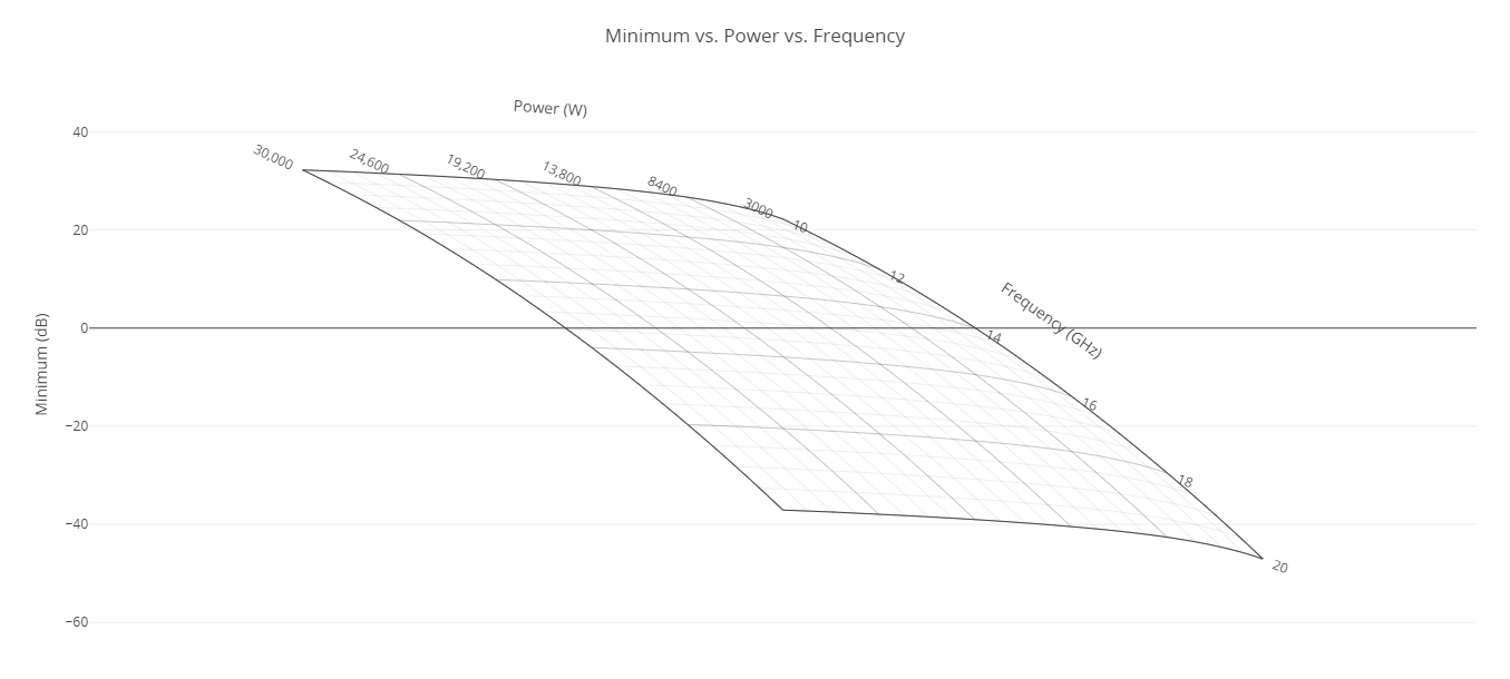
Minimum Eb/No Vs. Power Vs. Frequency Carpet plot
Optimizing the transmitter parameters
You now know that transmitter parameters have a large impact on coverage capabilities. To optimize these parameters, you can either guess at values or employ an optimization tool. Although you can clearly see trends from the previous studies, guessing at values will be difficult because you are dealing with multiple parameters at the same time and the trends you have studied thus far assume only one or two parameters are changed at a time. To solve more complex problems, the STK Analyzer Optimization capability, by means of the ModelCenter software's Optimization tool, can be a very useful guide. The Optimization tool is a collection of optimization algorithms that you can use within the ModelCenter application. A common graphical user interface (GUI) is provided to define optimization problems. An algorithm selection wizard is also provided to make it easy to choose algorithms that will work best for the problem at hand.
Creating an objective
Objective functions can be specific variables or equations composed of multiple output variables. Your objective is to minimize the value for power by changing frequency, data rate, and power all while maintaining a minimum Eb/No value of as close to 0 to 10 dB as possible.
- Click Optimization Tool (
 ) in the Standard toolbar.
 - Click and drag Power () from the Component Tree to the Objective field when the Optimization tool opens.
- Ensure the Goal field is set to Minimize.
Setting the constraints
Constraints restrict particular variables to a region or value.
- Click and drag Minimum () to the Constraint field.
- Set the Lower Bound to 0 and the upper bound to 10.
Selecting the Design Variables
The design variables are the variables that the optimizer will modify to meet the objective.
- Click and drag Power (), Frequency (), and DataRate () from the Component Tree to the Design Variable field.
- Set the following Design Variable values:
| Design Variable | Lower Bound | Upper Bound |
|---|---|---|
| Power | 300 | 30000 |
| Frequency | 10 | 20 |
| DataRate | 10e+06 | 20e+06 |
Selecting the algorithm
Many algorithms are available, including gradient-based optimizers, genetic algorithms, multiobjective algorithms, and other heuristic search methods.
- Select DAKOTA CONMIN methods in the Algorithm drop-down list.
- Click .
- Close the 2D Scatter Plot that automatically opened after the trade study finished running.
The DAKOTA (Design Analysis Kit for Optimization and Terascale Applications) toolkit provides a flexible and extensible interface between computational models and iterative analytical methods. CONMIN is a gradient-based optimizer that uses the method of feasible direction to solve constrained problems.
The optimizer will display a history of steps as it progresses. By default, it will display only the objective definition.
Viewing the results
When the optimization study is complete, you can view the convergence history of the process and see the best design.
- Return to the Optimization tool.
- Click on the Optimization tool panel to reveal the convergence history of the process.
- Select the Best Design tab, which contains the optimized values, when the Optimization tool Results window opens. These values are also displayed in the Value column for the design variables in the Optimization tool.
- Close the Optimization tool Results window when you are finished.
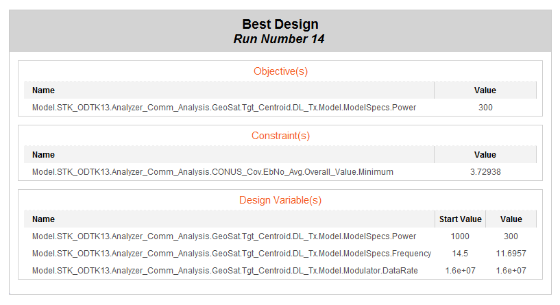
Best Design
The optimizer was able to drive power to its lower bound of 300 watts while at the same time attaining the goal of between 0 and 10 decibels of minimum Eb/No for the duration.
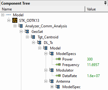
Reviewing your optimized workflow
With your model optimized, review your the updated values.
- Return to your ModelCenter Workspace.
- Take note of the updated values of your input values. You will need them in the next section.
- Close out any open plots and the Data Explorer window.
- Click when prompted to close your trade study without saving.
- Click Save (
 ) to save your ModelCenter workflow and to keep ModelCenter open.
Updated values
Updating the values in your STK scenario
Now that your transmitter specs are optimized, update those properties in your STK scenario.
- Reopen the Analyzer_Comm_Analysis scenario in the STK application ().
- Right-click on DL_Tx ().
- Select Properties (
 ) in the shortcut menu.
 - Ensure the Model Specs tab is selected when the Properties Browser opens.
- Enter the optimized Frequency value in the Frequency field, rounded to four decimal points (for example, 11.6957 GHz).
- Enter the optimized Power value in the Power field (for example, 300 W).
- Enter the optimized Data Rate in the Data Rate field (for example, 16 Mb/sec).
- Click to accept your changes and to close the Property Browser.
Recomputing coverage
With your transmitter model specs updated, recompute coverage.
- Right-click on CONUS_Cov ().
- Select CoverageDefinition in the shortcut menu.
- Select ComputeAccesses in the CoverageDefinition submenu.
Regenerating the Grid Stats report
Generate a new Grid Stats report to see how the values have changed.
- Right-click on EbNo_Avg () in the Object Browser.
- Select Report & Graph Manager... () in the shortcut menu.
- Select the Grid Stats () report in the Installed Styles () folder.
- Click .
- Review the Grid Stats report.
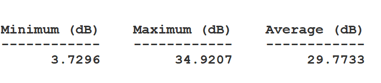
Final Grid Stats Report
Your FOM properties are very close to the ideally optimized values. You can also compare your 2D Graphics view with the original legend.
Updated Coverage over CONUS
Note that while the Eb/No closer to the center of the transmitter's boresight has decreased, the overall quality of coverage across CONUS has increased.
Saving your work
Save your work and close out of the STK and ModelCenter applications.
- Close out of any open reports and tools.
- Click Save () to save your scenario.
- Close the STK application.
- Return to the ModelCenter application ().
- Close out any open plots and the Data Explorer window.
- Click when prompted to close your trade study without saving.
- Click Save () to save your ModelCenter workflow.
- Close the ModelCenter application.
Summary
You began by reviewing the coverage of a transmitter attached to a satellite in GEO over the contiguous United States in a prebuilt scenario. Using the ModelCenter application, you ran a series of parametric studies to better understand how the transmitter's model specs affected the quality of coverage. Next, you created a carpet plot to better understand the combinations of frequency and power desired that gave you a minimum coverage capability of at least 0 dB for the coverage area. Finally, you optimized your transmitter model specs to minimize the value for power by changing frequency, data rate, and power all while maintaining a minimum Eb/No value of as close to 0 to 10 dB as possible and refreshed the results to visualized its improved coverage capability.