STK Premium (Air), STK Premium (Space), or STK Enterprise
You can obtain the necessary licenses for this tutorial by contacting AGI Support at support@agi.com or 1-800-924-7244.
Required product install: The Ansys ModelCenter® model-based systems engineering software and the STK Plugin for ModelCenter are required to complete this tutorial.
ModelCenter installation prerequisites: The ModelCenter software requires the installation of a 64-bit version of Java, a 64-bit implementation of Python 3.x, and the installation of the thrift and six Python packages. See the ModelCenter Installation Prerequisites for more information.
This tutorial was written using version 2026 R1 of the Ansys ModelCenter® model-based systems engineering software.
The results of the tutorial may vary depending on the user settings and data enabled (online operations, terrain server, dynamic Earth data, etc.). It is acceptable to have different results.
Capabilities covered
This lesson covers the following capabilities of the Ansys Systems Tool Kit® (STK®) digital mission engineering software:
- STK Pro
- Coverage
- Communications
- STK Analyzer
Problem statement
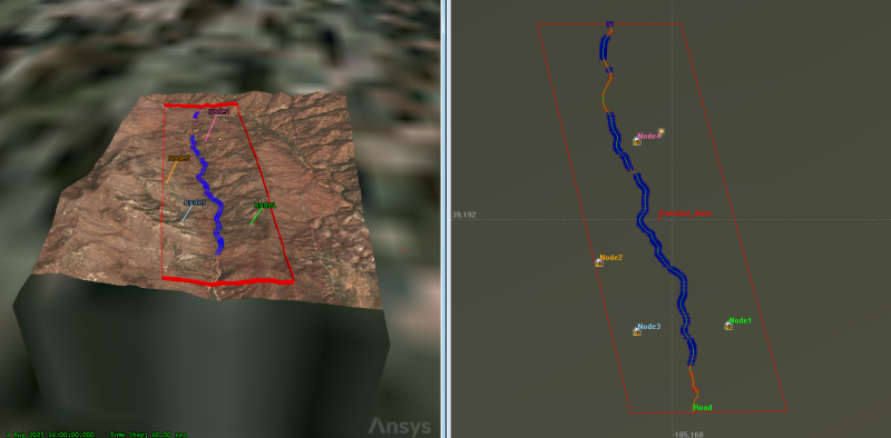
Engineers and operators want study the impact of terrain on a communications link to a ground vehicle traveling on a road through an exercise area located in mountainous terrain. There are four proposed locations for communication nodes that could be used as relays to a satellite and finally to a receiving station. You want to assess the impact of the communication node antenna height on the ability to communicate with the ground vehicle along the entirety of the road's path.
Solution
Use the Analyzer capability, which is part of the Ansys ModelCenter® model-based systems engineering software, to first create a carpet plot to see the impact of changing two antennas at a time. Then, use the Design of Experiments tool to vary the height of all four antennas at the same time to find the best possible configuration for all the antennas.
What you will learn
Upon completion of this tutorial, you will understand the following:
- Analyze a scenario for trends
- Use ModelCenter's Design of Experiments tool to vary two or more parameters in your scenario and observe the impact on an output
Using the starter scenario
To speed things up and allow you to focus on the portion of this exercise that teaches you how to use the ModelCenter software, a partially created scenario has been provided for you.
Opening the starter scenario
The starter scenario is included in your install.
- Launch the STK application (
 ).
). - Click
 Open a Scenario in the Welcome to STK dialog box.
 - Browse to <Install Dir>\Data\Resources\stktraining\VDFs.
- Select NodeHeight.vdf.
- Click .
Saving the VDF as a scenario file
Save and extract the VDF data in the form of a scenario folder. When you save a VDF in the STK application, it will save in its originating format. That is, if you open a VDF, the default save format will be a VDF (.vdf). If you want to save and extract a VDF as a scenario folder, you must change the file format by using the Save As feature. This will create a permanent scenario file complete with child objects and any additional files packaged with the VDF.
- Open the File menu when the starter scenario opens.
- Select Save As....
- Select the STK User folder in the navigation pane when the Save As dialog box opens.
- Select the NodeHeight folder.
- Click .
- Select Scenario Files (*.sc) in the Save as type drop-down list.
- Select the NodeHeight scenario file in the file browser.
- Click .
- Click in the Confirm Save As Dialog box to overwrite the existing scenario file in the folder and to save your scenario.
A scenario folder with the same name as the VDF was created for you when you opened the VDF in the STK application. This folder contains the temporarily unpacked files from the VDF.
When saving a VDF containing external files as a scenario folder, you must extract its contents to the scenario folder the STK application automatically creates for you in the STK User folder. This allows files packaged with the VDF, such as data files, reports, presentations, HTML pages, scripts, spreadsheets, and other files, to unpack to the scenario folder. If you save the VDF as a scenario folder in another location, these additional files will not be included. See the
Save (![]() ) often during this lesson!
) often during this lesson!
Computing coverage statistics
You will use the ModelCenter software's Design of Experiments tool to perform trade studies on the Percent Satisfied report for a Figure of Merit. Before creating the report, you must first manually compute the data in the STK application. The STK software's
The scenario consists of an Area Target object, called Exercise_Area, four Facility objects (Node1, Node2, Node3, and Node4) grouped in a Constellation object, called Nodes, to represent possible communication sites, and a Line Target object, called Road, representing the mountain road. A Coverage Definition object, Node_Cov, uses Road as its selected boundary object, the Constraints Facility object as its grid constraint, and the Nodes Constellation object as its assigned assets.
Computing accesses for the Node_Cov coverage area
First, compute the accesses along the route for the Node_Cov Coverage Definition object.
- Right-click on Node_Cov (
 ) in the Object Browser.
 - Select CoverageDefinition in the shortcut menu.
- Select Compute Accesses in the CoverageDefinition submenu.
Computed Access
Generating a Percent Satisfied report
A Percent Satisfied report presents the percentage of the total grid area and actual area where the static value a Figure Of Merit meets the specified satisfaction criterion.
- Right-click on the HowsMyCov Figure of Merit (FOM) (
 ) under the Node_Cov object in the Object Browser.
 - Select the Report & Graph Manager... (
 ) in the shortcut menu.
 - Expand (
 ) the Installed Styles (
 ) folder in the Styles pane when the Report & Graph Manager opens.
 - Select the Percent Satisfied (
 ) report.
 - Click .
In the resulting report, note the % Satisfied value. This value will be accessible in ModelCenter as an output variable.
Creating a new ModelCenter project
The
- Save (
 ) your scenario.
 - Close any open reports, the Report & Graph Manager, and any open tools.
- Close the STK application.
- Open the ModelCenter (
 ) application.
 - Click in the Welcome to ModelCenter dialog box.
- Click when the What type of model would you like to create? dialog box opens.
- Navigate to your scenario folder (for example, C:\Users\<username>\Documents\STK_ODTK 13\NodeHeight.
- Enter NodeHeight in the File name field.
- Ensure the Save as type is set to the ModelCenter Model (Zip) (*.pxcz).
- Click .
Configuring the STK Plugin for ModelCenter
The
- Select favorites (
 ) in the Server Browser at the bottom of the window.
 - Click and drag the STK component (
 ) into the dashed circle underneath "Drop items here to build the model" in the workspace.
 - Select NodeHeight.sc when the Open STK Scenario file dialog box opens.
- Click .
- After a few moments, the STK Analyzer window will open.
The NodeHeight scenario file will open in the STK application in the background.
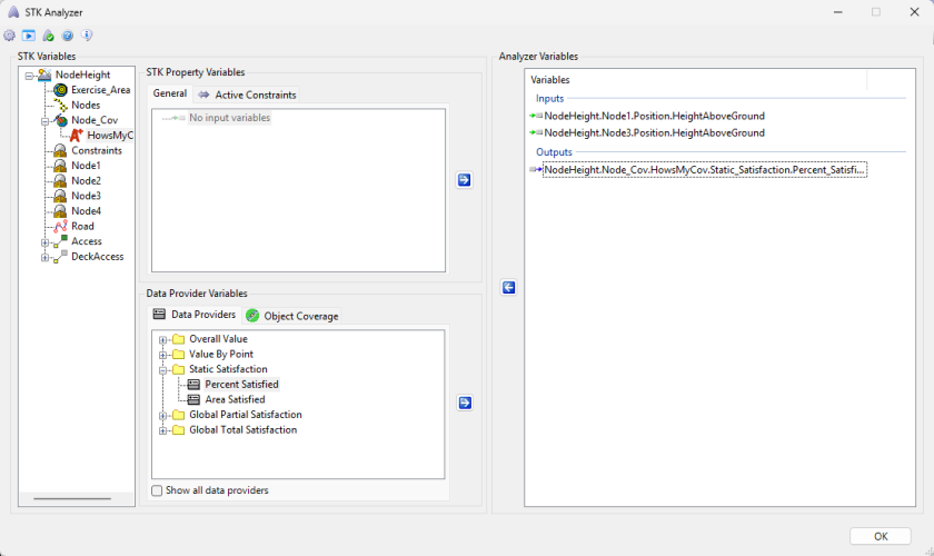
You can add any of the STK variables as ModelCenter input or output variables through the STK Analyzer window that appears. If you change the value of a variable in your scenario through the STK interface or the ModelCenter Component Tree, you should re-add the variable into ModelCenter or re-run the workflow before running any trade studies with the new value.
Assessing the impact of changing two antenna heights with Analyzer
Use the STK Analyzer window to configure the input and output variables available for further analysis with the
Selecting the Analyzer input variables
You will first run a Carpet Plot to analyze the impact of raising the height of two of the antennas. You could choose any pair of antennas you would like; for this study, you will look at Node1 and Node3.
- Select Node1 (
 ) in the STK Variables tree.
 - In the STK Property Variables tree, expand (
 ) the Position (
 ) property.
 - Select HeightAboveGround (
 ).
). - Move (
 ) HeightAboveGround () to the Analyzer Variables list.
 - Select Node3 ().
- In the STK Property Variables tree, expand () the Position () property.
- Select HeightAboveGround ().
- Move () HeightAboveGround () to the Analyzer Variables list.
When you select an object in the STK Variables tree, all possible input variable candidates for that object are listed under the General tab and the Active Constraints tab in the STK Property Variables panel.
It will show up under the Inputs list.
Both HeightAboveGround variables are listed as Inputs in the Analyzer Variables list.
Selecting the Analyzer output variable
The same data providers that are available in the Report & Graph Manager in the STK application are available in the Data Provider Variables tree.
- Expand () Node_Cov () in the STK Variables tree.
- Select HowsMyCov ().
- In the Data Provider Variables tree, expand () the Static Satisfaction (
 ) data provider.
 - Select the Percent Satisfied data provider element (
 ).
). - Move () Percent Satisfied () to the Analyzer Variables list.
- Click to confirm your selections and to close the STK Analyzer window.
The Percent Satisfied variable is listed under Outputs in the Analyzer Variables list.
STK Analyzer main form
This will also close the STK application, which had been running in the background.
Building a Carpet Plot
A Carpet Plot is a means of displaying data dependent on two variables in a format that makes interpretation easier than normal multiple curve plots. A Carpet Plot can be thought of as a multi-dimensional Parametric Study. To perform a Carpet Plot study, you must specify two design variables and a response. For the design variables, you must specify a starting value, ending value, and number of steps. To select variables, drag them from the Component Tree and drop them into the Carpet Plot tool.
- Expand () all the elements in the Component Tree.
- Click Carpet Plot (
 ) in the Standard toolbar.
 - Click and drag Node1's HeightAboveGround (
 ) variable into the first Design Variables field when the Carpet Plot tool opens.
 - Click and drag Node3's HeightAboveGround () variable to the second Design Variables field.
- Set the following values for both inputs:
- Click and drag Percent_Satisfied (
 ) into the Responses field.
| Option | Value |
|---|---|
| From | 0 |
| To | 0.1 |
| Num Steps | 4 |
Note that the HeightAboveGround values are in kilometers. The Step Size will adjust automatically.
Carpet Plot tool
When you run a trade study, it will first build a table of runs. These runs consist of all combinations of the two design variables for their specified ranges and number of steps. After the table has been created, it will run through each case and store values in the Data Explorer.
- Click to run the trade study.
- Once the trade study is complete and all data have been collected in the Data Explorer, the Carpet Plot displays.
- Review the Carpet Plot.
Note that no plots will appear for this study until all data points have been collected. The total number of runs is the multiplication of the two step values; for example, specifying step values of 4 and 4 will result in a total of 16 runs.
You can see the full variable names by clicking Toggle Full Variable Names in the view controls in the upper-right corner of the plot window.
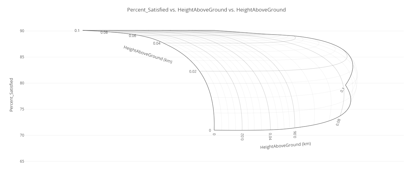
NodeHeight Carpet Plot
Adding a Contour Plot
There are multiple views that can be selected to visualize the data seen on the Table page. For this exercise, you will also add a Contour Plot. A Contour Plot measures the effects of 2 independent variables on a given variable, but does so in a 2D fashion, using color to represent the range of values the dependent variable is in, like a topographical map.
- Click Add View (
 ) on Carpet Plot toolbar.
 - Select Contour Plot (
 ) in the drop-down menu.
 - Review the Contour Plot.
- Close all data open plots and the Data Explorer window when you are finished.
- Click when prompted to close your trade study without saving.
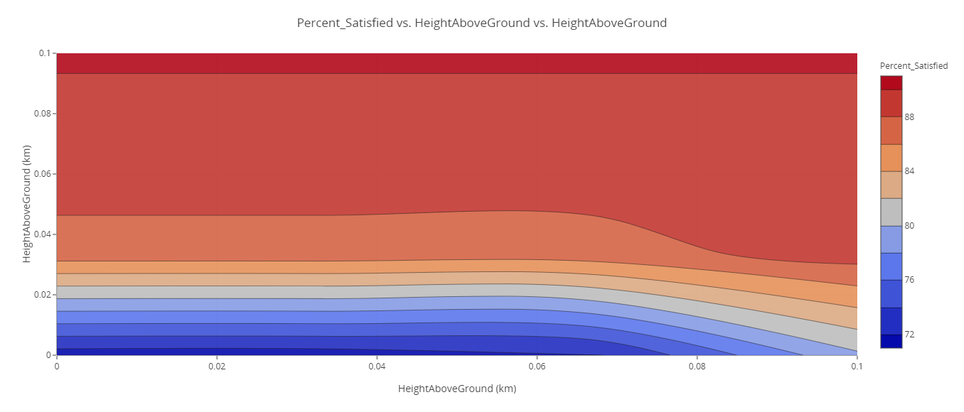
NodeHeight Contour Plot
The Carpet and Contour Plots indicate that changing Node3's height has a much greater impact on the percent of the road covered than Node1.
Varying all four antenna heights using the Design of Experiments tool
You've seen the impact of varying two antenna heights. The Carpet Plot showed that varying Node1's height had less impact on coverage time than varying Node3's height. By using the Design of Experiments tool, you'll be able to see how each of the nodes impact coverage time. The DOE (Design of Experiments) Tool simplifies the purposeful changing of inputs (design variables) in a model to observe the corresponding changes in outputs (response variables). A set of valid values for each design variable constitutes a design point. Use this tool to collect the responses in the model to a set of predetermined design points. Tools are provided to graphically set up and conduct this experiment.
Adding additional design variables
Add the HeightAboveGround variables from the other two antennas to your ModelCenter analysis.
- Right-click on the STK_ODTK13 component in the Analysis View.
- Select Show Component's GUI (
 ) in the shortcut menu.
 - Select Node2 ().
- In the STK Property Variables tree, expand () the Position () property.
- Move () HeightAboveGround () to the Analyzer Variables list.
- Select Node4 ().
- In the STK Property Variables tree, expand () the Position () property.
- Move () HeightAboveGround () to the Analyzer Variables list.
- Click .
This will open the STK scenario and STK Analyzer windows. Please be patient; this may take a while.
It will show up under the Inputs list.
Using the Design of Experiments tool
DOE tests contain two types of variables. A design variable is an input to a model that possibly affects the critical response variables. The critical response variables are the factors of the model that the user is trying to gain an understanding of (either to minimize or maximize the response to the design variables). To perform a DOE, the user must specify a set of design and response variables. For each design variable, the user must also specify an upper and lower value.
- Expand () all the elements in the Component Tree.
- Click DOETool (
 ) on the Standard toolbar.
 - Click and drag Node1's HeightAboveGround () variable to the Design Variables field when the Design of Experiments tool opens.
- Repeat the step above for the Node2, Node3, and Node4 HeightAboveGround () variables.
- Set the following values for all four Design Variables values:
- Click and drag Percent_Satisfied () into the Response Variables field.
| Option | Value |
|---|---|
| Low | 0 |
| High | 0.1 |
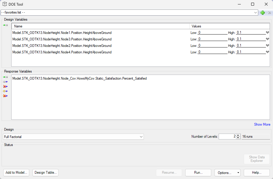
DOE Tool
Running the DOE trade study
When the DOE study is run, it will repeatedly set the value for the design variables and then validate each of the response variables. At each iteration it will store the values in the Model in the Data Explorer.
- Click to perform the DOE study.
- Examine the results in the Data Explorer.
After scrolling through the table of results, you can see that the best possible coverage percentage is approximately 95%. It is interesting to note that this amount of coverage can be achieved with only two antennas raised to 100 m. This occurs with the combination of Node1 and Node2 as well as the combination of Node2 and Node3, each raised to 100 m.
Creating a Variable Importance Summary Plot
A Variable Importance Summary Plot allows you to see which individual design parameters (main effects) and combinations of design parameters (interaction effects) have the most influence on the currently selected output variable. This plot helps you to quickly zero in on the most important design parameters for your problem.
- Click Add View () on the Table Page toolbar.
- Select Variable Importance Summary Plot (
 ) in the drop-down menu.
 - Hover over the topmost bar to see the full variable name.
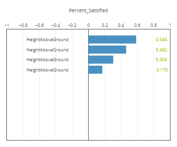
Variable Importance Summary plot
The Variable Importance Summary Plot shows that Node2 has the greatest effect on the overall coverage, whereas Node1 has the least. You could use this information to further refine your model to reduce the number of design variables in your overall problem, gain a better understanding of the design space, and to better estimate regions of good designs.
Saving your work
Save your work and close out ModelCenter application.
- Close out any open plots, tools, and the Data Explorer window.
- Click when prompted to close your trade study without saving.
- Click Save (
 ) to save your ModelCenter workflow.
 - Close the ModelCenter application.
Summary
Using a prebuilt scenario, you computed access between a constellation of four communication nodes along a route through mountainous terrain and determined the overall satisfaction using a Figure of Merit object. Using the STK Plugin for ModelCenter, you imported the node height and satisfaction data providers from your scenario into the ModelCenter model-based systems engineering software. You then created a Carpet Plot and a Contour Plot using two of the Node height variables, which showed that changing one Node's height had a greater impact on the coverage satisfaction than the other. Finally, you performed a Design of Experiment test on all four Node heights and generated a Variable Importance Summary Plot, which showed that Node2's height had the greatest impact on the overall coverage compared to the other node locations.