STK Premium (Space) or STK Enterprise
You can obtain the necessary licenses for this tutorial by contacting AGI Support at support@agi.com or 1-800-924-7244.
Required product install: The Ansys ModelCenter® model-based systems engineering software and the STK Plugin for ModelCenter are required to complete this tutorial.
ModelCenter installation prerequisites: The ModelCenter software requires the installation of a 64-bit version of Java, a 64-bit implementation of Python 3.x, and the installation of the thrift and six Python packages. See the ModelCenter Installation Prerequisites for more information.
This tutorial was written using version 2026 R1 of the Ansys ModelCenter® model-based systems engineering software.
The results of the tutorial may vary depending on the user settings and data enabled (online operations, terrain server, dynamic Earth data, etc.). It is acceptable to have different results.
Capabilities covered
This lesson covers the following capabilities of the Ansys Systems Tool Kit® (STK®) digital mission engineering software:
- STK Pro
- Astrogator
- STK Analyzer
Problem statement
Engineers and mission planners want to analyze the relationship between Delta-V and the time it takes for a probe to get from a low-Earth orbit into a low-altitude lunar orbit. You not only want to minimize the Delta-V of the maneuver, but you also want to keep the transfer time within an acceptable range.
Solution
Use the STK/Astrogator® capability and the Analyzer capability, which is part of the Ansys ModelCenter® model-based systems engineering software, to perform a parametric study to determine which duration of the translunar injection (TLI) maneuver delivers the lowest Delta-V. Then. perform another trade study to see how the required thrust changes when launching over different days.
Using the starter scenario
To speed things up and allow you to focus on the portion of this exercise that teaches you how to use the ModelCenter software, a partially created scenario has been provided for you.
Opening the starter scenario
The starter scenario is included in your install.
- Launch the STK application (
 ).
). - Click
 Open a Scenario in the Welcome to STK dialog box.
 - Browse to <Install Dir>\Data\Resources\stktraining\VDFs.
- Select Analyzer_LunarMission.vdf.
- Click .
Saving the VDF as a scenario file
Save and extract the VDF data in the form of a scenario folder. When you save a VDF in the STK application, it will save in its originating format. That is, if you open a VDF, the default save format will be a VDF (.vdf). If you want to save and extract a VDF as a scenario folder, you must change the file format by using the Save As feature. This will create a permanent scenario file complete with child objects and any additional files packaged with the VDF.
- Open the File menu when the starter scenario opens.
- Select Save As....
- Select the STK User folder in the navigation pane when the Save As dialog box opens.
- Select the Analyzer_LunarMission folder.
- Click .
- Select Scenario Files (*.sc) in the Save as type drop-down list.
- Select the Analyzer_LunarMission scenario file in the file browser.
- Click .
- Click in the Confirm Save As Dialog box to overwrite the existing scenario file in the folder and to save your scenario.
A scenario folder with the same name as the VDF was created for you when you opened the VDF in the STK application. This folder contains the temporarily unpacked files from the VDF.
When saving a VDF as a scenario folder, you should extract its contents to the scenario folder the STK application automatically creates for you in the STK User folder. See the
Save (![]() ) often during this lesson!
) often during this lesson!
Reviewing the starter scenario
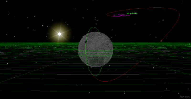
The Lunar Probe is launched into a Low Earth Orbit (LEO) transfer orbit and propagates until the trans-lunar injection burn. After the burn, it is further propagated until it reaches perilune, the point at which a spacecraft in lunar orbit is closest to the moon. At that time, another burn is performed to place the Lunar Probe into orbit around the Moon. Take a moment to familiarize yourself with the starter scenario.
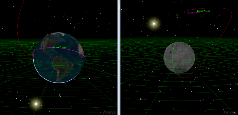
Lunar Probe 3D Graphics windows
Viewing the Launch Segment
The
- Right-click on LunarProbe (
 ) in the Object Browser.
 - Select Properties (
 ).
). - Select Launch (
 ) in the MCS.
 - Note that Epoch in the Launch panel is set to 0.0000000 EpDay.
Your scenario's analysis period is one epoch year, and your launch is set to occur at the very beginning of your analysis period. You will vary the launch epoch later in this tutorial.
Understanding the Target Moon Target Sequence
A
- Select the Target Moon (
 ) Target Sequence in the Mission Control Sequence.
 - Note that there are two differential corrector profiles for Target Moon.
- Select Differential Corrector in the Profiles field.
- Click Properties... () in the Profiles toolbar.
- Note the Control Parameters and the desired Equality Constraints (Results) when the Differential Corrector dialog box opens.
- Note the targeted duration of 259200 sec.
- Close the Differential Corrector dialog box without making any changes.
- Select Differential Corrector1 in the Profiles field.
- Click Properties... () in the Profiles toolbar.
- Note the Control Parameters and the desired Equality Constraints (Results).
This Differential Corrector profile gets the satellite close to the Moon. It targets delta right ascension (Delta_Right_Asc) and delta declination (Delta_Decination) as well as the duration from the TLI maneuver until the satellite reaches the point of lunar orbit insertion.
You will analyze this three-day duration using ModelCenter.
The second differential corrector profile targets the B-plane and gets the satellite into the desired lunar orbit. Note that the value of BDotR is 5000 km to avoid having the orbit intersect the Moon.
Use the Astrogator capability to build a mission to the Moon and learn more about B-plane targeting in the
Changing the differential corrector
Make a change with this second differential corrector before moving on.
- Under Equality Constraints (Results), change the desired value of BDotR to 6000 km.
- Click to confirm your changes and to close the Differential Corrector dialog box.
- Click Run Entire Mission Control Sequence (
 ).
). - Close each of the target status windows.
Three target status windows will appear that inform you of the results of each differential corrector run. There is a differential corrector for Establish Lunar Orbit that places the Lunar Probe in a circular orbit.
Updated 6,000 km BDotR
Creating a dependent variable for use in ModelCenter
In this exercise, you want to change the time of flight and determine the required TLI Delta-V.
- Return to the MCS.
- Select burn (
 ), nested within the Target Moon () Target Sequence in the MCS.
 - Click below the MCS.
- Expand (
 ) Maneuver (
 ) in the Available Components list.
 - Select DeltaV (
 ).
). - Click Insert Component (
 ).
). - Click to confirm your change and to close the User-Selected Results dialog box.
- Click to confirm your change and to close the Properties Browser.
Clicking this button opens the User-Selected Results dialog box, in which you can view and select calculation objects for Astrogator to report and target when defining a Differential Corrector Target Sequence profile. In this case, you are targeting the true altitude above Earth.
Creating a new ModelCenter project
The
- Save (
 ) your scenario.
 - Close the STK application.
- Open the ModelCenter (
 ) application.
 - Click in the Welcome to ModelCenter dialog box.
- Click when the What type of model would you like to create? dialog box opens.
- Navigate to your scenario folder (for example, C:\Users\<username>\Documents\STK_ODTK 13\Analyzer_LunarMission.
- Enter Analyzer_LunarMission in the File name field.
- Ensure the Save as type is set to the ModelCenter Model (Zip) (*.pxcz).
- Click .
Launching the STK Plugin for ModelCenter
The
- Select favorites (
 ) in the Server Browser at the bottom of the window.
 - Click and drag the STK component (
 ) into the dashed circle underneath "Drop items here to build the model" in the workflow's Analysis View.
 - Select Analyzer_LunarMission.sc when the Open STK Scenario file dialog box opens.
- Click .
- After a few moments, the STK Analyzer window will open.
The Analyzer_LunarMission scenario file will open in the STK application in the background.
You can add any of the STK variables as ModelCenter input or output variables through the STK Analyzer window that appears. If you change the value of a variable in your scenario through the STK interface or the ModelCenter Component Tree, you should re-add the variable into ModelCenter or re-run the workflow before running any trade studies with the new value.
Setting up your analysis with Analyzer
Use the STK Analyzer window to configure the input and output variables available for further analysis with the
Selecting the Analyzer input variable
Your studies will focus on the Trip value (that is, the true anomaly) of the first propagate segment against the Delta-V of the maneuver segment. Select the Trip value as your input variable.
- Select LunarProbe () in the STK Variables tree.
- Expand (
 ) the Propagator (Astrogator) (
 ) property in the STK Property Variables tree.
 - Expand () the Target Moon () Target Sequence.
- Expand () the Profiles () property.
- Expand () the Differential_Corrector () property.
- Expand () the EqualityConstraints () property.
- Expand () the Duration () property.
- Select DesiredValue (
 ).
). - Move (
 ) DesiredValue () into the Analyzer Variables list.
When you select an object in the STK Variables tree, all possible input variable candidates for that object are listed under the General tab and the Active Constraints tab in the STK Property Variables panel.
Note that DesiredValue is listed under Inputs in the Analyzer Variables list.
Selecting the Analyzer output variables
Because you selected Delta-V to be calculated as a result for the differential corrector, it is available as an output variable in ModelCenter. Select it to add to your model.
- Return to Target Moon ().
- Expand () the burn (
 ) impulsive maneuver segment.
 - Expand () the Results () property.
- Select DeltaV (
 ).
). - Move () DeltaV () into the Analyzer Variables list.
- Click to confirm your selections and to close the STK Analyzer window.
Note that DeltaV is listed under Outputs in the Analyzer Variables list.
This will also close the STK application, which had been running in the background.
Determining the impact of Delta-V on the TLI burn duration
The first study you will perform plots the duration of the TLI against the Delta-V required.
Using the Parametric Study tool
The Parametric Study tool runs a workflow through a sweep of values for some input variable. You can plot the resulting data to view trends.
- Expand () all the elements in the Component Tree.
- Click Parametric Study (
 ) in the Standard toolbar.
 - Click and drag DesiredValue (
 ) from the Component Tree to the Design Variable field when the Parametric Study tool opens.
 - Set the following Design Variable values:
- Click and drag DeltaV (
 ) from the Component Tree to the Responses field.
 - Click .
| Option | Value |
|---|---|
| starting value | 200000 |
| ending value | 500000 |
| number of samples | 7 |
Note the step size is automatically set to 50000. The starting and ending values are in seconds. The computations can take a couple of minutes, so stick with a small number of steps for now. Setting the number of samples will determine step size; conversely, setting the step size will determine the number of samples.
Clicking will open the Data Explorer, which is a tool used by Trade Study tools to display data while they are being collected from the STK scenario. While data are being collected, the Data Explorer displays a progress meter, a halt button, and the data.
Creating a 2D Line Plot
Once the trade study is complete and all data have been collected, the Data Explorer toolbar becomes active. The Data Explorer stores values for all variables in a workflow and special variables from the trade study. Some trade study tools will automatically launch a default plot window when the trade study runs. For other plots, you can create them from the Add View menu. Any variable in the workflow can be plotted against any other variable. For this study, you will create a 2D Line Plot. A 2D Line Plot displays an X-Y plot for variables in your model.
- Close the 2D Scatter Plot that opened when the trade study finished running.
- Click Add View (
 ) on the Table Page toolbar.
 - Select 2D Line Plot (
 ) in the drop-down menu.
 - Review the 2D Line Plot.
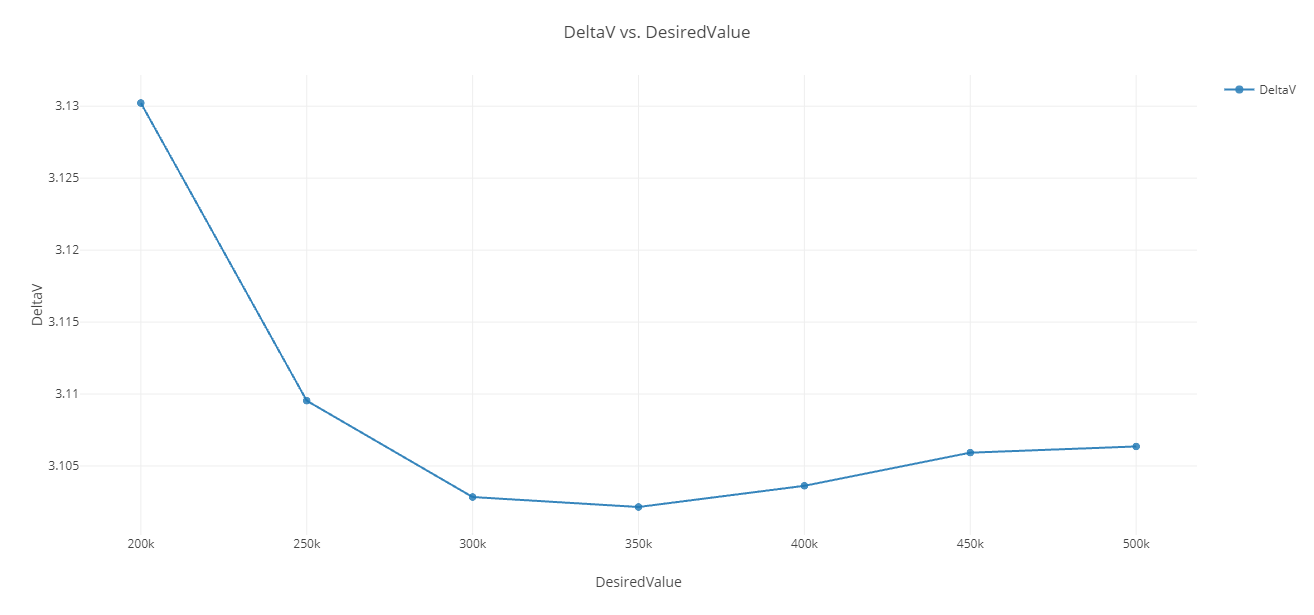
Delta-V vs Desired value
Closing out your trade study
Close out your trade study for the next section.
- Close the 2D Line Plot and the Table page when you are finished.
- Click when prompted to close your trade study without saving.
- Close the Parametric Study tool.
Studying the effect of launch epoch on Delta-V
The required thrust varies depending on the day on which the launch occurs. Using Analyzer's Carpet Plot Study Tool, vary the starting time by 30 days and analyze the amount of Delta-V required to reach the Moon over the course of a month.
Adding additional input variables
- Right-click on the STK_ODTK13 component in the Analysis View.
- Select Show Component's GUI (
 ) in the shortcut menu.
 - This will open the STK scenario and STK Analyzer windows.
- Select LunarProbe () in the STK Variables tree.
- Expand () the Propagator (Astrogator) () property in the STK Property Variables tree.
- Expand () the Target Moon () Target Sequence.
- Expand () the Launch () Launch segment.
- Select Launch_Epoch ().
- Move () Select Launch_Epoch () into the Analyzer Variables list.
- Click to confirm your selections and to close the STK Analyzer window.
Using the Carpet Plot tool
A Carpet Plot is a means of displaying data dependent on two variables in a format that makes interpretation easier than normal multiple curve plots. A Carpet Plot can be thought of as a multidimensional Parametric Study. Setting the design variables in a Carpet Plot is similar to using the Parametric Study tool, except you can study two variables simultaneously instead of one.
- Expand () all the elements in the Component Tree.
- Click Carpet Plot (
 ) on the Analyzer toolbar to access the Carpet Plot tool.
 - Click and drag DesiredValue () from the Component Tree to the first Design Variables field when the Carpet Plot tool opens.
- Set the following DesiredVlaue Design Variable values:
- Click and drag Launch_Epoch () from the Component Tree the second Design Variables field.
- Set the following Launch_Epoch Design Variable values:
- Click and drag DeltaV () from the Component Tree to the Responses field.
- Click .
- Close the Carpet Plot that is automatically generated after the trade study has finished running.
| Option | Value |
|---|---|
| From | 200000 |
| To | 500000 |
| Num Steps | 7 |
| Option | Value |
|---|---|
| From | 0.00000000 |
| To | 30 |
| Num Steps | 30 |
Note the step size is automatically set to 1.0345 day.
Because launch windows rarely occur at the same time each day, having your step size be slightly more than 24 hours will give you a good spread of values with far fewer failed runs compared to running with precise 24-hour steps.
You carpet plot will build over a series of 210 runs.
Be patient; this trade study may take several hours to complete.
Reviewing data in the Data Explorer
Review the runs of your model on the Table page. The Table page of the Data Explorer displays trade study data in a tabular form. It is the default window that is present for all trade studies. Cells are shaded differently depending on the associated variable's state. Input variables are shown with green text, valid values are displayed with black text, invalid values are displayed with gray text, and modified values are displayed with blue text. From the table it is possible to view and edit all values in your trade study and even to add and remove whole runs.
- Return to the Table page.
- Scroll through your table of runs.
- Note that several runs are colored red, which means they are invalid.

Table View with failed runs
In these instances, the differential correctors in your scenario's Target Sequences did not converge with the selected input variables, and so the run failed. You would not be able to launch at those times while meeting those targeted durations.
Creating a 3D Scatter Plot
A 3D Scatter plot displays an X-Y plot of variables in the workflow.
- Click Add View () on the Table Page toolbar.
- Select 3D Scatter Plot (
 ) in the drop-down menu.
 - Click Dimensions in the Plot Options menu when the 3D Scatter Plot opens.
- Open the color drop-down list.
- Select DeltaV.
- Click anywhere on the plot to close the Plot Options menu.
- Review the 3D Scatter Plot.
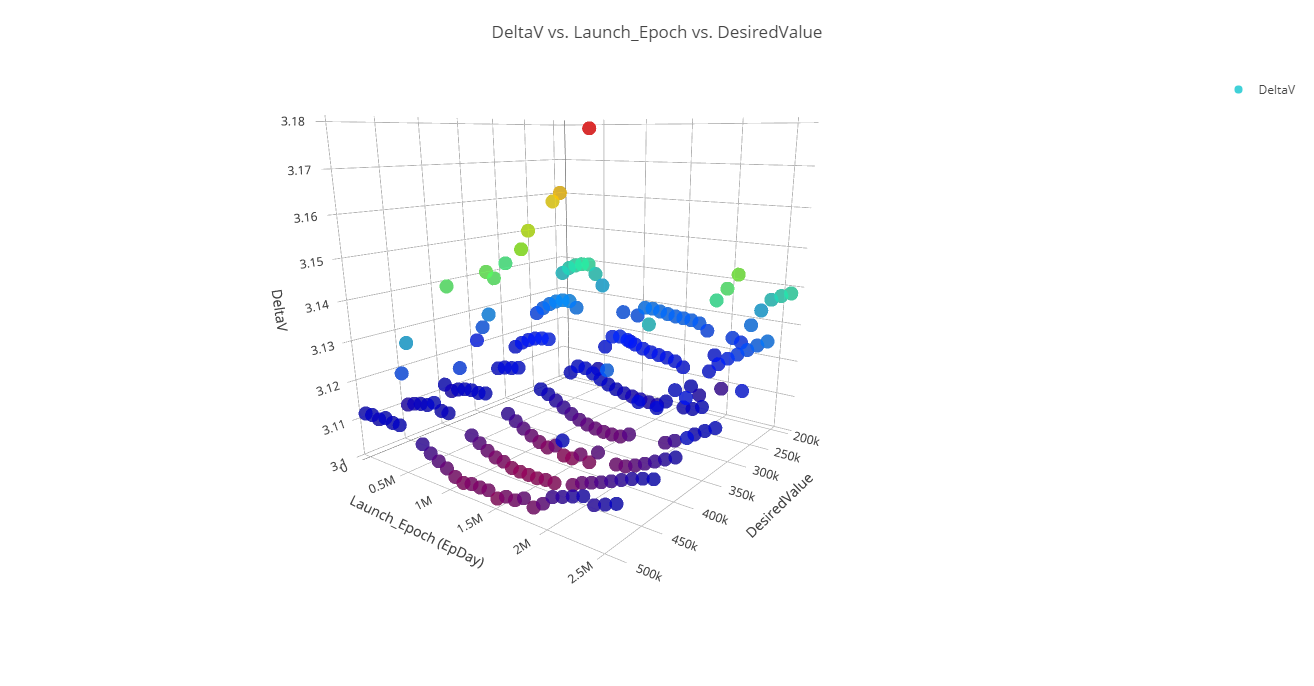
3D Scatter Plot of Delta-V vs. Launch Epoch Vs. Desired Value
You can see that at around 715,000 epoch seconds (about eight days), the required Delta-V spikes dramatically, but the period around 1.3-1.5 million epoch seconds (about 15-17 days) requires the least Delta-V to achieve lunar orbit during those 30 days.
Creating an Interactions Effects Plot
An Interactions Effects Plot shows quantitatively how the selected output variable changes (on average) as each of the two design parameters is varied from its lower bound to its upper bound. The influence of all other design parameters is averaged out.
- Click Add View () on the 3D Scatter Plot toolbar.
- Select Interactions Effects Plot (
 ) in the drop-down menu.
 - Click Dimensions in the Plot Options menu when the Interactions Effects Plot opens.
- Open the x drop-down list.
- Select Launch_Epoch.
- Open the y drop-down list.
- Select DesiredValue.
- Click anywhere on the plot to close the Plot Options menu.
- Review the plot.
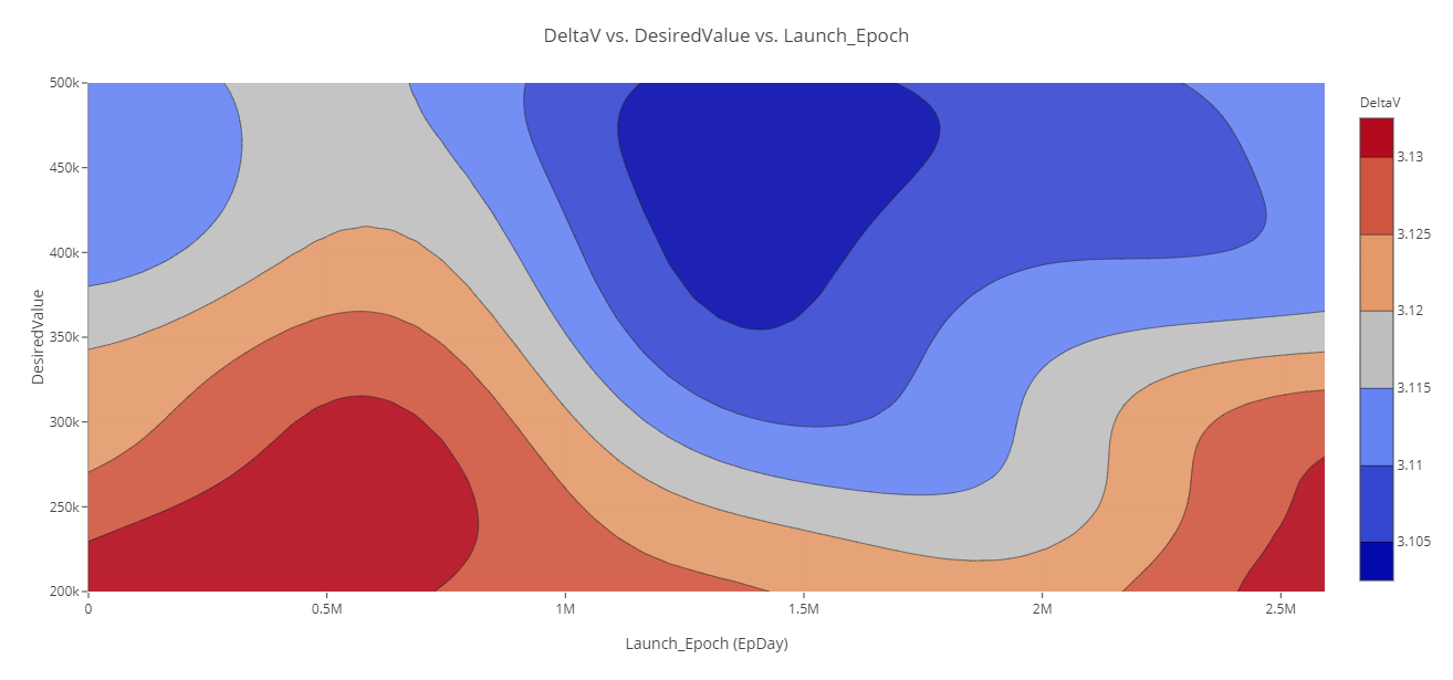
Interaction Effects Plot of Delta-V vs. Desired Value Vs. Launch Epoch
You can see that the most consistent region with the lowest Delta-V is around the same time (15-17 days from the start of the epoch), centered around a desired value of 450,000 seconds. While the study did not provide information for specific launch windows during those periods, you can use the study to narrow a range of launch days to better meet your mission requirements.
Saving your work
Save your work and close out ModelCenter application.
- Close out any open plots, tools, and the Data Explorer window.
- Click when prompted to close your trade study without saving.
- Click Save (
 ) to save your ModelCenter workflow.
 - Close the ModelCenter application.
Summary
You began by opening a prebuilt scenario of a lunar probe launching from earth and entering lunar orbit, which was propagated using the Astrogator capability. Using the ModelCenter software, you examined the Target Sequence surround the trans-lunar injection maneuver to understand the variables you are studying. You then studied the duration of the TLI maneuver and its effect on the resulting Delta-V required for successful insertion into lunar orbit. Finally, you studied the impact launching on different days had on the Delta-V requirements.