STK Premium (Air), STK Premium (Space), or STK Enterprise
You can obtain the necessary licenses for this tutorial by contacting AGI Support at support@agi.com or 1-800-924-7244.
Required product install: The Ansys ModelCenter® model-based systems engineering software and the STK Plugin for ModelCenter are required to complete this tutorial.
ModelCenter installation prerequisites: The ModelCenter software requires the installation of a 64-bit version of Java, a 64-bit implementation of Python 3.x, and the installation of the thrift and six Python packages. See the ModelCenter Installation Prerequisites for more information.
This tutorial was written using version 2026 R1 of the Ansys ModelCenter® model-based systems engineering software.
The results of the tutorial may vary depending on the user settings and data enabled (online operations, terrain server, dynamic Earth data, etc.). It is acceptable to have different results.
Capabilities covered
This lesson covers the following capabilities of the Ansys Systems Tool Kit® (STK®) digital mission engineering software:
- STK Pro
- Coverage
- STK Analyzer
- STK Analyzer Optimization
Problem statement
Engineers and operators require a quick way to determine how various orbital parameters will affect the ability of a sensor or camera to view the surface of the Earth. Your team wants to launch a satellite into low Earth orbit (LEO) to monitor the extent of Arctic sea ice. Data will be relayed through a GEO satellite back to a ground processing facility in Montreal. You want to understand what effects changing the satellite's orbital parameters and the configuration of its onboard sensor will have on it ability to view the polar ice cap.
Solution
Use the STK software's Coverage capability and the Analyzer capability, which is part of the Ansys ModelCenter® model-based systems engineering software, to perform a series of trade studies to better understand how the LEO satellite's orbit and sensor parameters impact coverage. Then, use the STK Analyzer Optimization capability to optimally configure the satellite's orbit and sensor to maximize the extent of coverage over the Arctic ice pack.
What you will learn
Upon completion of this tutorial, you will understand how to:
- Parametrically explore the design space in order to optimize your mission
- Perform parameter studies that vary an input variable through a range of values
- Plot one or more output variables
- Analyze an STK scenario for trends
- Generate 3D surface plots and perform optimization studies
- Optimize scenario parameters to meet mission objectives
Using the starter scenario
To speed things up and allow you to focus on the portion of this exercise that teaches you how to use the ModelCenter software, a partially created scenario has been provided for you.
Opening the starter scenario
The starter scenario is included in your install.
- Launch the STK application (
 ).
). - Click
 Open a Scenario in the Welcome to STK dialog box.
 - Browse to <Install Dir>\Data\Resources\stktraining\VDFs.
- Select SensorOpt.vdf.
- Click .
Saving the VDF as a scenario file
Save and extract the VDF data in the form of a scenario folder. When you save a VDF in the STK application, it will save in its originating format. That is, if you open a VDF, the default save format will be a VDF (.vdf). If you want to save and extract a VDF as a scenario folder, you must change the file format by using the Save As feature. This will create a permanent scenario file complete with child objects and any additional files packaged with the VDF.
- Open the File menu when the starter scenario opens.
- Select Save As....
- Select the STK User folder in the navigation pane when the Save As dialog box opens.
- Select the SensorOpt folder.
- Click .
- Select Scenario Files (*.sc) in the Save as type drop-down list.
- Select the SensorOpt scenario file in the file browser.
- Click .
- Click in the Confirm Save As Dialog box to overwrite the existing scenario file in the folder and to save your scenario.
A scenario folder with the same name as the VDF was created for you when you opened the VDF in the STK application. This folder contains the temporarily unpacked files from the VDF.
When saving a VDF as a scenario folder, you should extract its contents to the scenario folder the STK application automatically creates for you in the STK User folder. See the
Save (![]() ) often during this lesson!
) often during this lesson!
Reviewing the starter scenario
The starter scenario consists of your satellite of interest, LEO, with an attached simple conic sensor, Ice_Finder, which has a Ground Sample Distance (GSD) of five meters, as you want to be able to resolve icebergs as small as five meters in diameter. The Arctic region it is studying is represented by a Coverage Definition object, Arctic_Monitor. Arctic_Monitor's grid area of interest is the Area Target object named Arctic; the grid is constrained by a Facility object, Seed, which is not displayed in the 3D Graphics window, and the quality of coverage is gauged by a Figure Of Merit object, CoveragePerDay. Arctic_Monitor's assigned asset is Relay_Chain, a Chain object. Animate the scenario to view the Chain object's links from the ground station in Montreal through the GEO_Relay to LEO and LEO's Ice_Finder sensor.
- Click Start (
 ) to animate the scenario.
 - View LEO (
 ) as it scans the polar ice cap.
 - Click Reset (
 ) when you are finished.
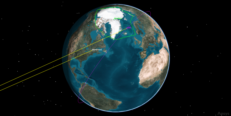
LEO viewing polar ice cap
Using the Coverage capability for analysis
The STK software's Coverage capability allows you to analyze the global or regional coverage provided by one or more assets (facilities, vehicles, sensors, etc.) while considering all accesses. To address area coverage capabilities, Coverage provides you with two STK object classes: Coverage Definition objects and Figure of Merit objects. Before running a Coverage analysis, however, you must first insert a Coverage Definition object.
Using the Compute Accesses tool
The ultimate goal of the STK software's Coverage capability is to analyze accesses to an area using assigned assets and applying necessary limitations upon those accesses. Compute coverage with the Compute Accesses tool.
- Right-click on Arctic_Monitor (
 ) in the Object Browser.
 - Select CoverageDefinition in the shortcut menu.
- Select Compute Accesses in the CoverageDefinition submenu.
Generating a Grid Stats report
The scenario has a seven-day analysis period. CoveragePerDay's definition is set to Coverage Time and computing option is Per Day. Per Day is the total coverage time divided by the number of days in the coverage interval. You will use the ModelCenter software to perform trade studies on CoveragePerDay's Grid Stats. First, manually collect data in the STK application by generating a Grid Stats report to see the smallest to largest number of accesses to any point in the grid.
- Right-click on CoveragePerDay (
 ) in the Object Browser.
 - Select Report & Graph Manager... (
 ) in the shortcut menu.
 - Select the Grid Stats (
 ) report in the Installed Styles (
 ) folder.
 - Click .
- Note the Minimum, Maximum, and Average values in the report. These values will be accessible in Analyzer as output variables.
- Close the Grid Stats report when you are finished.
- Close the Report & Graph Manager.
- Save (
 ) your scenario.
 - Close the STK application.
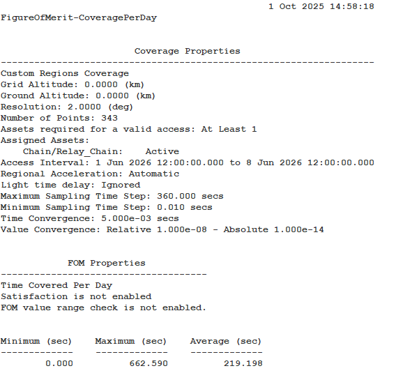
Grid Stats Report
This report indicates that for all the grid points defining the polar cap, at least one point is not seen by the satellite (Minimum = 0.000), at least one point is seen for approximately 663 seconds, and on average, points are seen for approximately 219 seconds per day during your analysis period.
Creating a new ModelCenter project
The
- Open the ModelCenter (
 ) application.
 - Click in the Welcome to ModelCenter dialog box.
- Click when the What type of model would you like to create? dialog box opens.
- Navigate to your scenario folder (for example, C:\Users\<username>\Documents\STK_ODTK 13\SensorOpt.
- Enter SensorOpt in the File name field.
- Ensure the Save as type is set to the ModelCenter Model (Zip) (*.pxcz).
- Click .
Launching the STK Plugin for ModelCenter
The
- Select favorites (
 ) in the Server Browser at the bottom of the window.
 - Click and drag the STK component (
 ) into the dashed circle underneath "Drop items here to build the model" in the workflow's Analysis View.
 - Select SensorOpt.sc when the Open STK Scenario file dialog box opens.
- Click .
- After a few moments, the STK Analyzer window will open.
The SensorOpt scenario file will open in the STK application in the background.
You can add any of the STK variables as ModelCenter input or output variables through the STK Analyzer window that appears. If you change the value of a variable in your scenario through the STK interface or the ModelCenter Component Tree, you should re-add the variable into ModelCenter or re-run the workflow before running any trade studies with the new value.
Setting up your analysis with Analyzer
Use the STK Analyzer window to configure the input and output variables available for further analysis with the
Selecting the Analyzer input variables
Your first study will focus on several of the satellite's orbital parameters, such as Inclination, RAAN, and the Semi-major Axis, as input variables. Before you can use them in your model, however, you must first add them to your design space.
- Select LEO () in the STK Variables tree.
- Expand (
 ) the Propagator (J4Perturbation) (
 ) property in the STK Property Variables tree.
 - Move (
 ) the following input variables (
 ) to the Analyzer Variables list:
 - SemiMajorAxis
- Inclination
- RAAN
When you select an object in the STK Variables tree, all possible input variable candidates for that object are listed under the General tab and the Active Constraints tab in the STK Property Variables panel.
Note that all three variables are listed as Inputs in the Analyzer Variables list.
Selecting the output variables
The same data providers that are available in the Report & Graph Manager in the STK application are available in the Data Provider Variables tree.
- Expand () Arctic_Monitor () in the STK Variables tree.
- Select CoververagePerDay ().
- Expand () the Overall Value (
 ) data provider in the Data Provider Variables tree.
 - Move () the following data provider elements (
 ) into the Analyzer Variables list.
 - Minimum
- Maximum
- Average
- Click to confirm your selections and to close the STK Analyzer window.
Note that the variables are listed as Outputs in the Analyzer Variables list.
This will also close the STK application, which had been running in the background.
Analyzing the effects of inclination on coverage
You want to understand how LEO's inclination affects its ability to monitor the Arctic region. Create a Parametric Study to plot the inclination against the coverage time per day.
Using the Parametric Study tool
The Parametric Study tool runs a workflow through a sweep of values for some input variable. You can plot the resulting data to view trends.
- Expand (
 ) all the elements in the Component Tree.
 - Click Parametric Study (
 ) in the Standard toolbar.
 - Click and drag Inclination (
 ) from the Component Tree to the Design Variable field when the Parametric Study tool opens.
 - Set the following Design Variable values:
- Click and drag Minimum (
 ), Maximum (), and Average () from the Component Tree to the Responses field.
 - Click .
| Option | Value |
|---|---|
| starting value | 45 |
| ending value | 135 |
| step size | 10 |
Clicking will open the Data Explorer, which is a tool used by Trade Study tools to display data while they are being collected from your Model. While data are being collected, the Data Explorer displays a progress meter, a halt button, and the data. The Table page of the Data Explorer displays trade study data in a tabular form. It is the default window that is present for all trade studies. Cells are shaded differently depending on the associated variable's state. Input variables are shown with green text, valid values are displayed with black text, invalid values are displayed with gray text, and modified values are displayed with blue text. From the table it is possible to view and edit all values in your trade study and even to add and remove whole runs.
Creating a 2D Line Plot
Once the trade study is complete and all data have been collected, the Data Explorer toolbar becomes active. The Data Explorer stores values for all variables in a workflow and special variables from the trade study. Some trade study tools will automatically launch a default plot window when the trade study runs. For other plots, you can create them from the Add View menu. For this study, you will create a 2D Line Plot. A 2D Line Plot displays an X-Y plot for variables in your model. Any variable in the workflow can be plotted against any other variable.
- Close the 2D Scatter Plot that opened when the trade study finished running.
- Click Add View (
 ) on the Table Page toolbar.
 - Select 2D Line Plot (
 ) in the drop-down menu.
Setting the plot variables
The plot shows the minimum coverage time versus the inclination. You could change the plot's y dimension to maximum or average to adjust the plot as needed. Instead, you will add the maximum and average coverage results to the plot for comparison on one plot. Use the Plot Options menu to set which variable is displayed on which axis. In certain plots, you can set other global plot controls based on the plot variables. In this case, you want to view several variables: the minimum, maximum, and average power. Minimum will be Series 1, Maximum will be Series 2, and Average will be Series 3.
- Click Dimensions in the Plot Options menu on the left-hand side of the 2D Line Plot.
- Click Add Series (+).
- Set Series 2 - x to Inclination.
- Set Series 2 - y to Maximum.
- Click Add Series (+).
- Set Series 3 - x to Inclination.
- Set Series 3 - y to Average.
- Click on the plot to close the Plot Options menu.
- Review the plot.
This adds the Maximum inclination values to the plot.
This adds the Average inclination values to the plot.
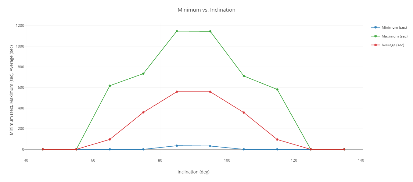
Minimum, Maximum, and average seconds vs. Inclination
Results from the first study are as expected: the closer the inclination is to 90 degrees, the better your coverage will be. This makes sense, as the ice cap covers the North Pole and your coverage will be best when your orbit takes you through the rotational center point of the area you are trying to cover.
There are two additional interesting trends in the data: the maximum coverage does not smoothly improve as inclination approaches 90 degrees, and more importantly, the minimum coverage value does not climb above zero until inclination reaches some value between 75 and 90 degrees.
Closing out your trade study
Close out your trade study for the next section.
- Close the 2D Line Plot and the Table page when you are finished.
- Click when prompted to close your trade study without saving.
- Leave the Parametric Study tool open.
Refining the trade study parameters
Since you want to ensure that your orbit will cover the entire ice cap, you want to run a more refined parametric study in the area of interest.
- Return to the Parametric Study tool.
- Set the following Design Variable values:
- Click .
| Option | Value |
|---|---|
| starting value | 85 |
| ending value | 95 |
| step size | 1 |
Reviewing the Table page data
While you can create line plots that are great for presentations or personal choice, you can also obtain the required information directly from the Table page.
- Close the 2D Scatter Plot that opened when the trade study finished running.
- Bring the Table page to the front when all runs finish.
- Examine the results.
- Close the Table page.
- Click when prompted to close your trade study without saving.
- Leave the Parametric Study tool open.
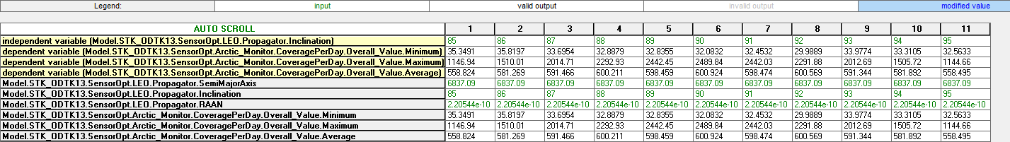
Table page
This study gives us a much better understanding of where to position the satellite to give you the best overall inclination to ensure maximum coverage of the whole ice cap. You can see that inclinations between 87 and 93 degrees will give you at least 2,000 seconds of maximum coverage of the ice cap during your analysis period.
Updating the inclination variable for further study
As noted earlier, the closer the inclination is to 90 degrees, the better your coverage will be. Set the inclination value to 90 for future studies so you can better understand the effects the other variables have on coverage.
- Click into the Inclination Value field in the Component Tree.
- Enter 90.
- Select the Enter key to set LEO's inclination to 90 degrees.
Determining the impact of RAAN on coverage
The satellite's RAAN (right ascension of the ascending node) might impact your coverage.
Running a new Parametric Study
Build a new Parametric Study using the satellite's RAAN as your Design Variable.
- Click and drag RAAN () from the Component Tree to the Design Variable field when the Parametric Study tool opens.
- Set the following Design Variable values:
- Click .
This will replace Inclination as the Design Variable.
| Option | Value |
|---|---|
| starting value | 0 |
| ending value | 360 |
| step size | 30 |
Reviewing the trade study data
Review the table data and create a 2D Line Plot to gain understanding of how the satellite's RAAN affects coverage.
- Bring the Table page to the front when all runs are completed.
- Close the 2D Scatter Plot that automatically opened after the trade study finished running.
- Use your cursor to expand the table of runs so that you can see all thirteen runs.
- Look at the data in the Table page.
- Click Add View () on the Table Page toolbar.
- Select 2D Line Plot () in the drop-down menu.
At first glance, the data appear to be fairly insensitive to RAAN. This may be due to the difference in scales minimum and maximum coverage values. To view just the minimum coverage values, create a new graph.
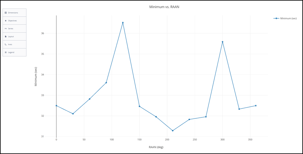
minimum seconds VS. RAAn
Minimum coverage values fluctuate for different RAAN values. This is an artifact of the low frequency sampling of the data. While the difference between high and low values is less than 10 percent of the mean, there are definitely some values that are better than others.
Closing out your trade study
Close out your trade study for the next section.
- Close the 2D Line Plot and the Table page when you are finished.
- Click when prompted to close your trade study without saving.
- Leave the Parametric Study tool open.
Determining the impact of the semi-major axis on coverage
The final orbit parameter impacting coverage is the satellite's semi-major axis. Vary the semi-major axis from 6,500 to 7,500 kilometers.
Running a new Parametric Study
Build a new Parametric Study using the satellite's RAAN as your Design Variable.
- Click and drag SemiMajorAxis () from the Component Tree to the Design Variable field when the Parametric Study tool opens.
- Set the following Design Variable values:
- Click .
- Close the 2D Scatter Plot that automatically opened after the trade study finished running.
- Click Add View () on the Table Page toolbar.
- Select 2D Line Plot () in the drop-down menu.
This will replace RAAN as the Design Variable.
| Option | Value |
|---|---|
| starting value | 6500 |
| ending value | 7500 |
| step size | 100 |
Updating the 2D Line Plot's variables
Adjust the 2D Line Plot's variables and examine it for trends.
- Click Dimensions in the Plot Options menu on the left-hand side of the 2D Line Plot.
- Click Add Series (+).
- Set Series 2 - x to SemiMajorAxis.
- Set Series 2 - y to Maximum.
- Click Add Series (+).
- Set Series 3 - x to SemiMajorAxis.
- Set Series 3 - y to Average.
- Click on the plot to close the Plot Options menu.
Reviewing the 2D Line Plot
With your series added, review the plot.
- Review the 2D Line Plot.
- Close the 2D Line Plot and the Table page when you are finished.
- Click when prompted to close your trade study without saving.
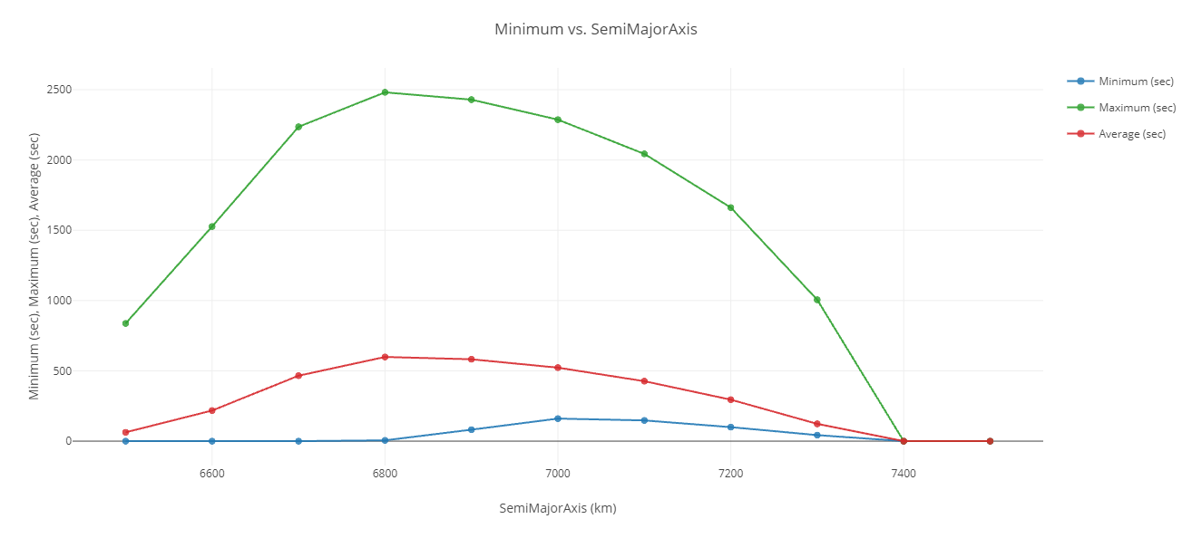
Minimum, Maximum, and average seconds vs. Semi-major Axis
There is an interesting trend here. The maximum and average coverage extents increase rapidly with the semi-major axis, but only until a certain point is reached; after that point, there is an equally sharp drop off. The minimum extent of coverage continues to increase even as the maximum and average extents of coverage decrease. This is due to a required five-meter
Studying the sensor's Ground Sample Distance
Limitations to a sensor's resolution can be defined in terms of its Ground Sample Distance. The Ground Sample Distance is the smallest size of an object on the ground that can be detected by the sensor. It is based upon the access geometry and the physical attributes of the sensor. The sensor is modeled as capturing an array of pixels, where each pixel has the same sized square shape when projected in front of the sensor. The sensor is also assumed to be pointed directly at the target. When the sensor is looking straight down on the target, the size of the pixel on the ground is simply the size of the square projected to the distance of the ground. As a single pixel is the smallest element of the image, this distance, which is denoted as the GSD, represents the smallest discernible feature size in the image.
The Sensor object's five-meter resolution can might have an impact on your trade study. Confirm this by rerunning the Parametric Study with the sensor's
Adding the constraint as an additional variable
Before you can study the impact of the Ground Sample Distance, you must add the constraint as a variable to your workflow.
- Right-click on the STK_ODTK13 component in the Analysis View.
- Select Show Component's GUI (
 ) in the shortcut menu.
 - Expand () LEO () in the STK Variables tree when the STK Analyzer window opens.
- Select Ice_Finder (
 ).
). - Select the Active Constraints tab in the STK Property Variables panel.
- Select GroundSampleDistance.max in the STK Property Variables tree.
- Move () GroundSampleDistance.max to the Analyzer Variables list.
- Click to confirm your changes and to close the STK Analyzer window.
This will open the STK scenario and STK Analyzer windows. Please be patient.
Note that GroundSampleDistance.max is now listed as an input variable.
Updating the Ground Sample Distance
Rather than removing the constraint entirely, you can use an extremely large number to effectively remove the maximum GSD constraint.
- In the Component Tree, expand () Ice_Finder (
 ).
). - Expand () GroundSampleDistance ().
- Click on the GroundSampleDistance - max value of 5.
- Enter 1e+300.
- Select the Enter key.
- Click Run (
 ) on the Standard toolbar to run the workflow and apply the changes.
 - Save (
 ) your ModelCenter project.
Rerunning the Parametric Study
With the GSD constraint effectively disabled, rerun the Parametric Study.
- Bring the Parametric Study tool () to the front.
- Click .
- Close the 2D Scatter Plot that automatically opened after the trade study finished running.
- Click Add View () on the Table Page toolbar.
- Select 2D Line Plot () in the drop-down menu.
- Close the 2D Line Plot and the Table page when you are finished.
- Click when prompted to close your trade study without saving.
- Close the Parametric Study Tool.
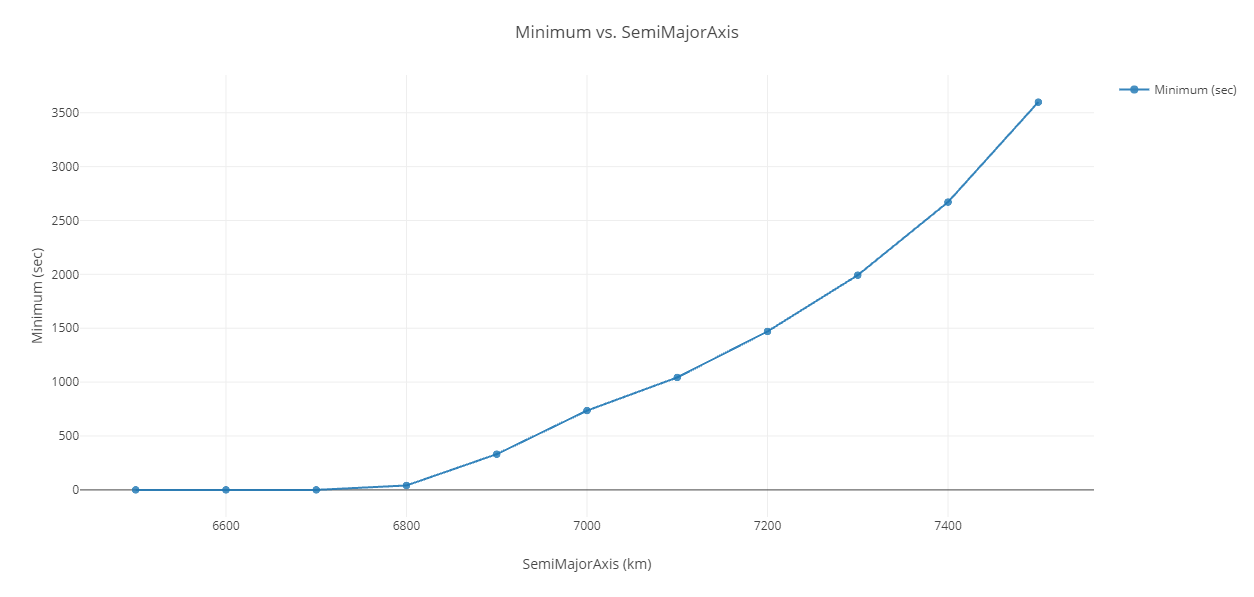
Minimum Seconds vs. Semi-major Axis without GSD Constraint
Not altogether surprisingly, the plot indicates that without a Ground Sample Distance constraint, as the semi-major axis increases, the extent of coverage also increases.
Resetting the Sensor object's Ground Sample Distance
Reset the Sensor object's Ground Sample Distance constraint for further trade studies.
- Click on the GroundSampleDistance - max value of 5.
- Enter 5.
- Select the Enter key.
- Click Run () on the Standard toolbar to run the workflow and apply the changes.
- Save () your ModelCenter project.
Analyzing the effect of semi-major axis and inclination together
You have determined that inclination and the semi-major axis have significant impacts on coverage capability while the RAAN has minimal influence. The semi-major axis had an increasingly positive impact until the Ground Sample Distance constraint came into effect. Coverage generally improves as inclination approaches 90 degrees. This leads to two questions: Does changing the semi-major axis impact your conclusions about inclination? And can you improve your sensor characteristics to permit a higher orbit? Answer the first question by performing a multidimensional Parametric Study (Carpet Plot).
Using the Carpet Plot tool
A Carpet Plot is a means of displaying data dependent on two variables in a format that makes interpretation easier than normal multiple curve plots. A Carpet Plot can be thought of as a multidimensional Parametric Study. Setting the design variables in a Carpet Plot is similar to using the Parametric Study tool, except you now have two variables instead of one.
- Click Carpet Plot (
 ) on the Standard toolbar.
 - Click and drag Inclination () from the Component Tree to the first Design Variables field when the Carpet Plot tool opens.
- Set the following Inclination Design Variable values:
- Click and drag SemiMajorAxis () from the Component Tree to the second Design Variables field.
- Set the following SemiMajorAxis Design Variable values:
- Click and drag Average () from the Component Tree to the Responses field.
- Click .
- Close the Carpet Plot that automatically opened after the trade study finished running.
| Option | Value |
|---|---|
| From | 85 |
| To | 105 |
| Step Size | 5 |
| Option | Value |
|---|---|
| From | 6500 |
| To | 7500 |
| Step Size | 200 |
Creating a Main Effects Summary Plot
Create a Main Effects Summary Plot from the Table page to better visualize your trade study. A Main Effects plot shows quantitatively how the selected output variable changes (on average) as the design parameter is varied from its lower bound to its upper bound; the influence of the other design parameters is averaged out. A Main Effects Summary Plot show all the Main Effects Plots for both variables in the trade study.
- Bring the Table page to the front when all runs are completed.
- Click Add View () on the Table Page toolbar.
- Select Main Effects Summary Plot (
 ) in the drop-down menu.
 - Review the summary plots.
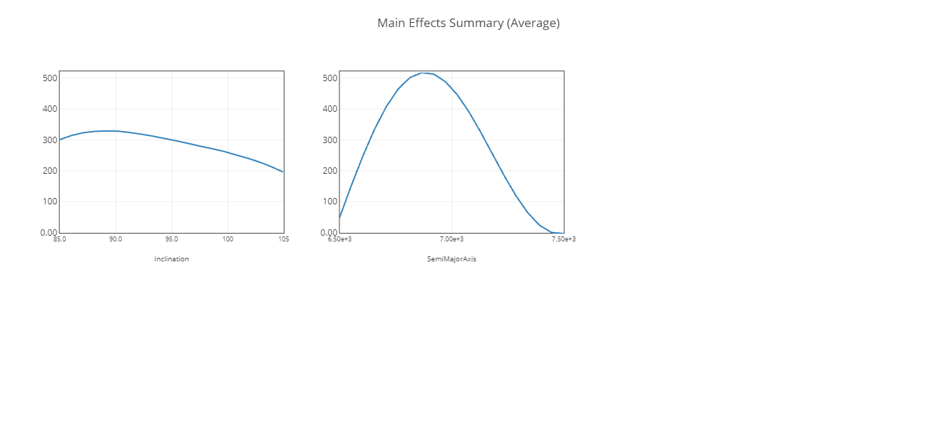
Main effects summary plots
The Main Effects Summary plot indicates that, regardless of the semi-major axis, the likely optimal inclination for the best average coverage time per day is around 90 degrees, and the semi-major axis is somewhere between 6,800 and 7,000 kilometers. The default semi-major axis value used in your scenario, 6837.09 km, would work nicely.
Closing out your trade study
Close out your trade study for the next section.
- Close Main Effects Summary Plot and the Table page when you are finished.
- Click when prompted to close your trade study without saving.
- Close the Carpet Plot tool.
Studying the sensor's resolution
You now know that for any given inclination, increasing the orbit's semi-major axis will improve coverage. However, you must take into account the five-meter Ground Sample Distance constraint for the Sensor object. You can study Ice_Finder's resolution properties to permit greater viewing capabilities at higher orbits, but you must first add the component variables, focal length and detector pitch, to your model.
- Right-click on the STK_ODTK13 component in the Analysis View.
- Select Show Component's GUI () in the shortcut menu.
- Expand () LEO () in the STK Variables tree when the STK Analyzer window opens.
- Select Ice_Finder ().
- Expand () the SimpleConic () property in the STK Property Variables tree.
- Select coneAngle ().
- Move () coneAngle () to the Analyzer Variables list.
- Select the Resolution () property in the STK Property Variables tree.
- Move () Resolution () to the Analyzer Variables list.
- Click to accept your changes and to close the STK Analyzer window.
This will add both FocalLength and DetectorPitch as input variables.
Studying the sensor's detector pitch
Determine the impact of varying the sensor's detector pitch on coverage.
Running a Parametric Study
Build a new Parametric Study using DeterctorPitch as your Design Variable. You will focus on maximum coverage for now.
- Expand () all the elements in the Component Tree.
- Click Parametric Study () in the Standard toolbar.
- Click and drag DetectorPitch () from the Component Tree to the Design Variable field.
- Set the following DetectorPitch Design Variable values:
- Click and drag Maximum () from the Component Tree to the Responses field.
- Click and from the Component Tree to the Responses field.
- Click .
| Option | Value |
|---|---|
| starting value | 0.0001 |
| ending value | 0.001 |
| step size | 0.0001 |
Creating a 2D Line Plot
Create a 2D Line Plot to investigate the data.
- Bring the Table page to the front when all runs are completed.
- Click Add View () on the Table Page toolbar.
- Select 2D Line Plot () in the drop-down menu.
- Click Axes in the Plot Options menu.
- Select the Ticks tab.
- Change the Max # value to 20.
- Click anywhere on the plot to close the Plot Options menu.
- Review the 2D Line Plot.
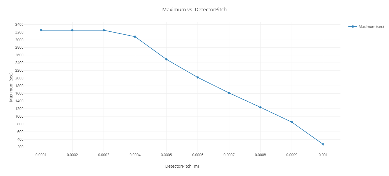
Maximum Seconds vs. Detector Pitch
Detector pitch has a maximum threshold value of approximately 0.0003 meter, which, if exceeded, will result in degraded coverage capabilities.
Closing out your trade study
Close out your trade study for the next section.
- Close the 2D Line Plot and the Table page when you are finished.
- Click when prompted to close your trade study without saving.
- Leave the Parametric Study tool open.
Studying the sensor's focal length
Determine the impact of focal length on coverage.
Running a Parametric Study
Build a new Parametric Study using FocalLength as your Design Variable.
- Return to the Parametric Study tool.
- Click and drag FocalLength () from the Component Tree to the Design Variable field.
- Set the following FocalLength Design Variable values:
- Click .
This will replace DetectorPitch as the Design Variable.
| Option | Value |
|---|---|
| starting value | 50 |
| ending value | 200 |
| step size | 10 |
Creating a 2D Line Plot
Create a 2D Line Plot to investigate the data.
- Bring the Table page to the front when all runs are completed.
- Click Add View () on the Table Page toolbar.
- Select 2D Line Plot () in the drop-down menu.
- Click Axes in the Plot Options menu.
- Select the Ticks tab.
- Change the Max # value to 20.
- Click anywhere on the plot to close the Plot Options menu.
- Review the 2D Line Plot.
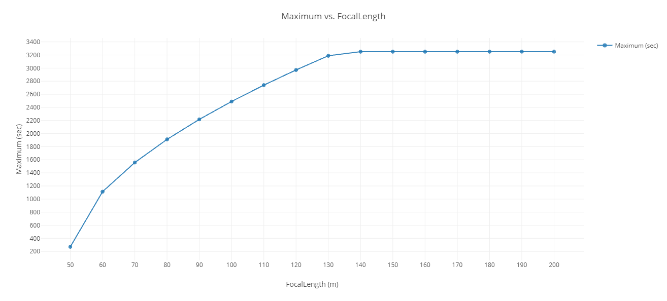
Maximum Seconds vs. Focal Length
The focal length has a threshold value of approximately 140 meters. After that, further increases don't improve coverage.
Closing out your trade study
Close out your trade study for the next section.
- Close the 2D Line Plot and the Table page when you are finished.
- Click when prompted to close your trade study without saving.
- Leave the Parametric Study tool open.
Studying the sensor's cone angle
Determine the impact of the cone angle sensor parameter.
Running a Parametric Study
Build a new Parametric Study using coneAngle as your Design Variable.
- Return to the Parametric Study tool.
- Click and drag coneAngle () from the Component Tree to the Design Variable field.
- Set the following coneAngle Design Variable values:
- Move Maximum from the Component Tree to the Responses list if needed
- Click .
| Option | Value |
|---|---|
| starting value | 20 |
| ending value | 60 |
| step size | 5 |
Creating a 2D Line plot
Create a 2D line plot to investigate the data.
- Bring the Table page to the front when all runs are completed.
- Click Add View () on the Table Page toolbar.
- Select 2D Line Plot () in the drop-down menu.
- Review the plot.
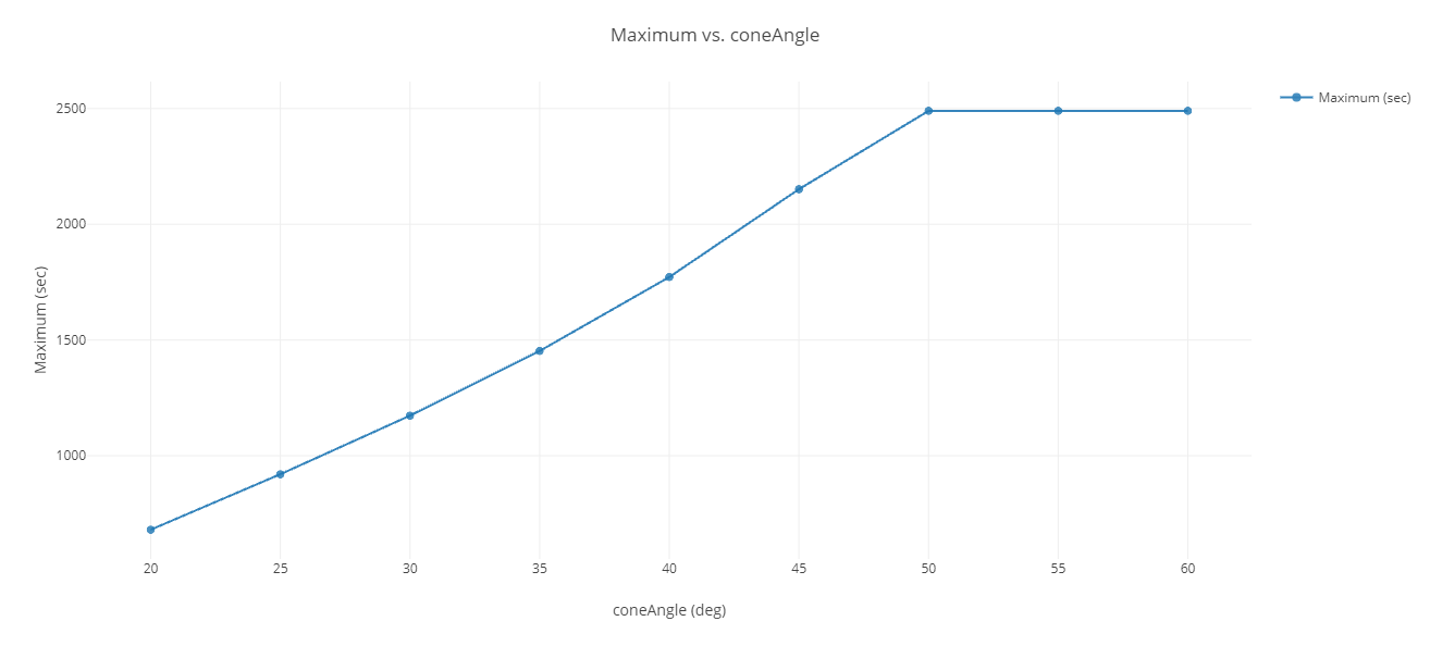
Maximum Seconds vs. Cone Angle
The cone angle has a threshold value of approximately 50 degrees.
Closing out your trade study
Close out your trade study for the next section.
- Close the 2D Line Plot and the Table page when you are finished.
- Click when prompted to close your trade study without saving.
- Close the Parametric Study tool open.
Optimizing the sensor with the Optimization tool
Sensor parameters have a large impact on coverage capabilities. Although you can see trends from the previous studies, guessing at values will be difficult because you are dealing with multiple parameters at the same time and the trends, thus far, assume only one or two parameters are changed at a time. To optimize these parameters, you can either guess at values or employ an Optimization tool. The Optimization tool is a collection of optimization algorithms that you can use within the ModelCenter application. A common graphical user interface (GUI) is provided to define optimization problems. An algorithm selection wizard is also provided to make it easy to choose algorithms that will work best for the problem at hand.
Use the STK Analyzer Optimization capability, by means of the ModelCenter software's Optimization tool, to minimize the focal length requirement for the sensor while maintaining a minimum coverage capability of 150 seconds per day for your coverage area.
Creating an objective
Objective functions can be specific variables or equations composed of multiple output variables.
- Click Optimization Tool (
 ) in the Standard toolbar.
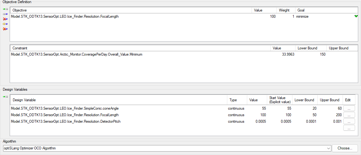
 - Click and Drag FocalLength () from the Component Tree to the Objective field on the right when the Optimization tool opens.
- Ensure the Goal is set to minimize.
Setting the constraints
Constraints restrict particular variables to a region or value.
- Click and drag Minimum () to the Constraint field.
- Set the Lower Bound to 150.
- Leave the Upper Bound blank.
Since there is no upper bound, you can leave it undefined.
Selecting the Design Variables
The design variables are the variables that the optimizer will modify to meet the objective. You want the optimizer to minimize the FocalLength by changing coneAngle, FocalLength, and DetectorPitch.
- Click and drag coneAngle (), FocalLength (), and DetectorPitch () from the Component Tree to first Design Variables field.
- Set the following Design Variable values:
| Design Variable | Start Value (Explicit Value) | Lower Bound | Upper Bound |
|---|---|---|---|
| coneAngle | 55 | 20 | 60 |
| FocalLength | 100 | 50 | 200 |
| DetectorPitch | 0.0005 | 0.0001 | 0.001 |
Note that each Start Value must be equal to or greater than its respective Lower Bound value. In this case, you are starting with your baseline detector parameters.
optimization tool values
Selecting the algorithm
Many algorithms are available, including gradient-based optimizers, genetic algorithms, multiobjective algorithms, and other heuristic search methods.
- Open the Algorithm drop-down list.
- Select optiSLang Optimizer OCO Algorithm.
- Click
- Note the Maximum number of design evaluations is set to 500 when the Options dialog opens.
- Click to close the Options Dialog without making any changes.
The Ansys ModelCenter software is integrated with five algorithms from the
The optiSLang One Click Optimizer (OCO) abstracts the complexity of optimization algorithms away from the end-user. Internally, numerous optimization algorithms and metamodels are used to find the best objective(s). OCO is an efficient hybrid optimization strategy that comes with only one major setting to be tuned: the maximum number of design evaluations. Depending on the type and number of input parameters and the defined optimization criteria, the optimizer automatically selects the most suitable optimization algorithms with their most appropriate settings to solve the optimization problem. The ability to dynamically switch between optimization algorithms and to run multiple algorithms simultaneously makes OCO one of the most reliable and efficient optimization strategies. OCO is a surrogate-assisted optimization strategy, using capabilities of the Metamodel of Optimal Prognosis (MOP) for function approximation to significantly speed up the optimization process.
This is the maximum number of design evaluations the algorithm will compute before stopping.
Running the optimization study
You are interested in the best design values.
- Click .
- View the 2D Scatter Plot that the Optimization tool automatically created for you.
- Close the 2D Scatter Plot when you are finished.
- Return to the Optimization tool.
- Click in the Status panel to show the convergence history of the process.
- Select the Best Design tab, which contains the optimized values, when the Optimization tool Results window opens. These values are also displayed in the Value column for the design variables in the Optimization tool.
- Close the Optimization tool Results window when you are finished.
Be patient. Your optimization study will take a while to complete.
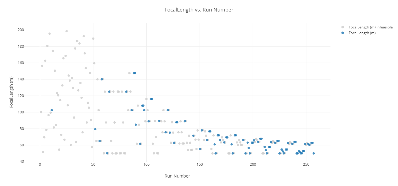
Optimization tool 2D Scatter Plot
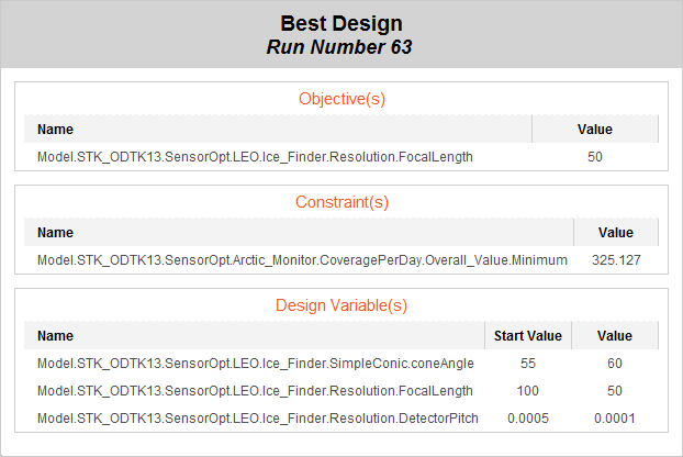
optimization tool Best design values
Your results for data values and best design run may be different from the above image. In this case, while the algorithm continued on and converged around a solution, the overall best value was from an earlier run.
After running an optimization study, the values in your model will be changed to the final, optimized values. In this case, your optimal minimum values were at the limits of your design specifications.
Saving your work
Save your work and close out ModelCenter application.
- Close out any open, plots, tools, and the Data Explorer window.
- Click when prompted to close your trade study without saving.
- Click Save () to save your ModelCenter workflow.
- Close the ModelCenter application.
Summary
You wanted to understand how a LEO satellite's orbital and sensor parameters impact coverage capabilities. Your solution for this problem was to optimally configure the satellite's orbit and sensor to best cover the polar ice cap. You did this by running a series of parametric studies. For each parametric study, you analyzed a single design parameter through a sweep of values. Next you created a carpet plot to view how multiple parameters impact coverage. Finally, you used the Optimization tool to scan through the design space to find a solution that met your requirements.