STK Premium (Space) or STK Enterprise
You can obtain the necessary licenses for this tutorial by contacting AGI Support at support@agi.com or 1-800-924-7244.
The results of the tutorial may vary depending on the user settings and data enabled (online operations, terrain server, dynamic Earth data, etc.). It is acceptable to have different results.
Capabilities covered
This lesson covers the following capabilities of the Ansys Systems Tool Kit® (STK®) digital mission engineering software:
- STK Pro
- Astrogator
Problem statement
A rendezvous and proximity operations (RPO) mission planner with minimal training wants to plan an RPO mission. RPO mission planning can be a very complex process. The STK/Astrogator® capability has a very robust feature set that allows for complex RPO mission planning and requires significant expertise to efficiently and effectively plan an RPO mission.
Solution
Use Astrogator to model an RPO mission. You will follow some basic steps in modeling missions of one satellite approaching another already in orbit using Astrogator. You will model two satellites already in the same plane, with a target satellite trailing the mission satellite in True Anomaly, and will target two in-plane burns to approach and subsequently circumnavigate the target satellite. You'll create a Mission Control Sequence (MCS) to perform a non-optimal transfer to the target satellite and a maneuver to enter into a Natural Motion Circumnavigation (NMC) relative orbit.
It is worth noting that there is nothing trivial about RPO. This tutorial is intended to address a common RPO mission requirement, while providing a basic understanding of Astrogator's techniques. It is not meant to cover or address all of the nuances regarding this type of relative orbit. As mentioned above, this tutorial will not result in a minimum Delta-V solution, as osculating orbital effects are not considered in determining optimal departure and transfer times.
Recommended training
This tutorial assumes you have some working knowledge of Astrogator. If not, you should go through the following tutorials to become familiar with Astrogator:
What you will learn
Upon completion of this tutorial, you will be able to:
- Model a target satellite and a maneuvering (RPO) satellite.
- Model a drift approach, Vbar hop, and target a NMC.
- Generate and evaluate relevant data sets.
Video guidance
Watch the following video. Then follow the steps below, which incorporate the systems and missions you work on (sample inputs provided).Creating a new scenario
First, you must create a new STK scenario, and then build from there.
- Launch the STK application (
 ).
). - Click
 Create a Scenario when the Welcome to STK dialog box opens.
 - Enter the following in the STK: New Scenario Wizard:
- Click when you finish.
- Click Save (
 ) when the scenario loads. The STK application creates a folder with the same name as your scenario for you.
 - Verify the scenario name and location in the Save As dialog box.
- Click .
| Option | Value |
|---|---|
| Name | LEO_Rendezvous |
| Location | Default |
| Start | Default |
| Stop | + 2 days |
Save (![]() ) often during this lesson!
) often during this lesson!
Adding the target satellite
Create your target satellite and propagate it using Astrogator.
Inserting a Satellite object
- Bring the Insert STK Objects tool (
 ) to the front.
 - Select Satellite (
 ) in the Select An Object To Be Inserted list.
 - Select Define Properties (
 ) in the Select A Method list.
 - Click .
Propagating the Satellite object using Astrogator
The Astrogator capability contains specialized analysis for interactive orbit maneuver and spacecraft trajectory design. Astrogator calculates the satellite's ephemeris by running a Mission Control Sequence, or MCS, that you define according to the requirements of your mission.
Astrogator enables you to model impulsive and finite maneuvers as well as high-fidelity orbit propagation. It provides targeting methods, including:
- A differential corrector used to find the necessary values of control parameters (such as launch epoch or burn duration) to meet desired mission goals.
- An optimizer used to change control parameters to achieve a goal, while applying a set of constraints that define the problem space.
Furthermore, Astrogator allows you to define automatic sequences. These represent predefined sets of actions that can be performed whenever a specified event occurs, such as a maneuver that occurs at every periapsis. These details highlight just some of Astrogator's many features.
Astrogator also utilizes a component catalog and editor in the STK application called the Component Browser. The
- Select the Basic - Orbit page when the Properties Browser opens.
- Open the Propagator drop-down list.
- Select Astrogator.
Setting up the MCS segments
MCS segments are the building blocks of an Astrogator space mission. There are two general types of segments: those that generate ephemeris and those that affect the execution of the MCS. These segments can be used interactively, so that ephemeris generated by one segment can change the way in which the MCS continues to run in a subsequent statement.
Selecting the Keplerian element coordinate type
Specify the shape and size of the satellite's orbit using the traditional ocscualting Keplerian orbital element coordinate type.
- Select Initial State (
 ) in the MCS.
 - Select the Elements tab.
- Open the Coordinate Type drop-down list.
- Select Keplerian.
Specifying the Keplerian elements
Now that you've set the Keplerian coordinate type, choose the element types and set their corresponding values.
- Open the Semi-major Axis drop-down list.
- Select Apoapsis Altitude.
- Enter 500 km in the Apoapsis Altitude field.
- Open the Eccentricity drop-down list.
- Select Periapsis Altitude.
- Enter 500 km in the Periapsis Altitude field.
- Enter 98.5 deg in the Inclination field.
- Enter 90 deg in the Right Asc. of Asc. Node field.
- Keep the remaining default values.
- Click to accept your changes and to keep the Properties Browser open.
Changing the Propagate segment's stopping condition
Use the Propagate segment to model the movement of the spacecraft along its current trajectory until meeting specified stopping conditions.
- Select Propagate (
 ) in the MCS.
 - Enter 2 day in the Trip field.
- Click to accept your changes.
Running the MCS
To calculate the trajectory of the spacecraft you must run the MCS. Astrogator will proceed through the MCS and run each segment, generating an ephemeris for the spacecraft. As it runs the MCS, Astrogator carries the trajectory and state of the spacecraft determined so far from one segment to the next.
- Click Run Entire Mission Control Sequence (
 ) in the MCS toolbar.
 - Click Clear Graphics (
 ) to remove iteration graphics after finishing the run.
 - Click to accept your changes.
Setting 2D and 3D Graphics window properties for space situational awareness
Set a 2D Graphics window property to enhance your space situational awareness. This is purely aesthetic.
- Select the 2D Graphics - Pass page.
- Click .
- Enter 10 sec in the Time between Orbit Points - Maximum field when the Pass Resolution Values dialog box opens.
- Click to accept your change and to close the Pass Resolution Values dialog box.
- Click to accept your changes and to close the Properties Browser.
Renaming the Satellite object
Rename the Satellite object.
- Right-click on Satellite1 () in the Object Browser.
- Select Rename in the shortcut menu.
- Rename Satellite1 () to Target_Sat.
Creating the RPO satellite
You have a good start on the RPO satellite with Target_Sat. Copy that satellite, then modify the copy's properties to model the RPO satellite.
Copying the target Satellite object
- Select Target_Sat () in the Object Browser.
- Click Copy (
 ) in the Object Browser toolbar.
 - Click Paste (
 ) in the Object Browser toolbar.
 - Rename Target_Sat1 () to RPO_Sat.
Modifying RPO_Sat's True Anomaly
Offset RPO_Sat 30 degrees ahead of Target_Sat in an in-plane leading position.
- Right-click on RPO_Sat () in the Object Browser.
- Select Properties () in the shortcut menu.
- Select the Basic - Orbit page when the Properties Browser opens.
- Enter 30 deg in the True Anomaly field in the Element Type list.
- Select Propagate () in the MCS.
- Click Segment Properties () in the MCS toolbar.
- Open the Color picker drop-down when the Edit Segment dialog box opens.
- Choose a different color than Target_Sat's () Propagate Segment.
- Click to accept your change and to close the Edit Segment dialog box.
- Click to accept your changes.
Running the MCS
Run RPO_Sat's MCS.
- Click Run Entire Mission Control Sequence () in the MCS toolbar.
- Click Clear Graphics ().
- Click to accept your changes.
Viewing the satellites in the 3D Graphics window
View the two propagated satellites in the 3D Graphics window.
- Bring the 3D Graphics window to the front.
- Use your mouse to set your view showing RPO_Sat () leading Target_Sat ().
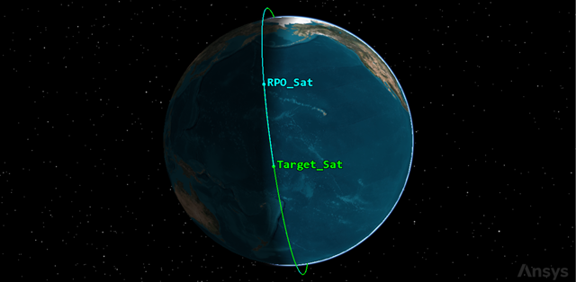
Target_Sat trailing rpo_sat
Referencing the target satellite
The Reference page of a satellite's basic properties enables you to specify a vehicle to be used as a reference vehicle in a formation flying situation with other satellites.
- Return to RPO_Sat's () Properties ().
- Select the Basic - Reference page.
- Select Target_Sat () in the Reference Vehicle list.
- Click .
- Click to accept your changes.
This sets the reference for relative parameters; for example, targeting relative orbit parameters.
Displaying RPO_Sat relative to Target_Sat
You can show the RPO_Sat trajectory relative to Target_Sat. This is an aesthetic change, but it makes the relative maneuvers easier to understand. To properly view RPO_Sat's orbit, make some changes to its 3D Graphics properties.
- Select the 3D Graphics - Pass page.
- Open the Lead Type drop-down list in the Orbit Track panel.
- Select All.
- Select the 3D Graphics - Orbit System page.
- Clear the Show check box for the Inertial by Window option.
- Click .
- Select Target_Sat () in the VVLH System Object list when the Select Object VVLH System dialog box opens.
- Click to close the Select Object VVLH System dialog box.
- Click to accept your changes.
This tells the 3D Graphics window to display the track spanning the entire vehicle ephemeris.
This is an object-centered Vehicle Velocity, Local Horizontal (VVLH) reference coordinate frame with the Z axis opposite the position vector and the X axis toward the inertial velocity vector.
Building the MCS to target Target_Sat
Modify RPO_Sat's MCS and build on it to maneuver and drift to the target satellite.
Adding an RPO maneuver to approach the target satellite
Add an RPO maneuver to RPO_Sat to get it close to Target_Sat.
- Select the Basic - Orbit page.
- Select Propagate () in the MCS.
- Enter 600 sec in the Trip field in the Stopping Conditions panel.
- Click to accept your changes.
This propagation time is an arbitrary selection based on an initial guess for a mission requirement, and may not be optimal. For an optimal (minimum Delta-V) solution, you can use a Lambert solver to seed a two-body initial guess to Astrogator (refer to the Design Tool Components topic for more information on the Lambert Solver). Conversely, you can use the optimization profiles of SNOPT or IPOPT within Astrogator. This will be discussed at the end of the tutorial.
Adding a Target Sequence
Use a Target Sequence as a structural element to define maneuvers and propagations in terms of the goals they are intended to achieve.
- Right-click on the Return Segment (
 ) in the MCS.
 - Select Insert Before... in the shortcut menu.
- Select Target Sequence (
 ) when the Segment Selection dialog box opens.
 - Click to accept your selection and to close the Segment Selection dialog box.
- Right-click on Target Sequence () in the MCS.
- Select Rename in the shortcut menu.
- Rename Target Sequence () to Target Approach.
Adding an in-plane maneuver
First you will insert an in-plane maneuver to cause the satellite to drift to a specific point (in RIC coordinates) relative to the target satellite.
- Right-click on the Return Segment () below Target Approach ().
- Select Insert Before... in the shortcut menu.
- Select Maneuver (
 ) when the Segment Selection dialog box opens.
 - Click to accept your selection and to close the Segment Selection dialog box.
Updating the Maneuver segment's properties
Update the Maneuver segment's properties.
- Right-click Maneuver () in the MCS.
- Select Properties... in the shortcut menu.
- Enter Burn1 in the Name field when the Edit Segment dialog box opens.
- Open the Color picker drop-down.
- Select white.
- Click to accept your changes and to close the Edit Segment dialog box.
Setting Burn1's thrust axes
Update Burn1's thrust axes to reference RPO_Sat's RIC coordinate frame.
- Select the Attitude tab.
- Open the Attitude Control drop-down list.
- Select Thrust Vector.
- Click the Thrust Axes ellipsis (
 ).
). - Open the Filter by drop-down list when the Select Reference dialog box opens.
- Select All Objects.
- Select RPO_Sat () in the object list.
- Select RIC (
 ) in the Axes for: RPO_Sat list.
 - Click to accept your change and to close the Select Reference dialog box.
Setting up the control parameters
Any element of a nested MCS segment or linked component that you can use as an independent variable is marked by a target icon (![]() ). To select an element as an independent variable, click its target icon. A check mark appears over the target (
). To select an element as an independent variable, click its target icon. A check mark appears over the target (![]() ). Click the target again to clear the selection of that element.
). Click the target again to clear the selection of that element.
- Select the following Cartesian targets (
 ).
). - X
- Y
- Z
- Keep the default values for each dimension (0 m/sec).
- Click to accept your changes.
This serves as the initial guess for the Target Sequence.
Drifting toward Target_Sat
Add a Propagate sequence to allow RPO_Sat to drift towards Target_Sat.
- Right-click Burn1 () in the MCS.
- Select Insert After... in the shortcut menu.
- Select Propagate () when the Segment Selection dialog box opens.
- Click to close the Segment Selection dialog box.
- Select Propagate () (under Burn1 () in the MCS.
- Click Segment Properties () in the MCS toolbar.
- Type Drift in the Name field when the Edit Segment dialog box opens.
- Open the Color picker drop-down.
- Select a different color from your other Propagate segments.
- Click to accept your changes and to close the Edit Segment dialog box.
Updating the stopping condition
Drift 30 degrees during a 10 hour duration or 3 degrees per hour.
- Select Drift () in the MCS.
- Enter 10 hr in the Trip field of the Stopping Conditions panel.
- Click to accept your changes.
- Click Run Entire Mission Control Sequence () in the MCS toolbar.
Similar to the propagation time above, this transfer duration is an arbitrary selection based the mission needs for this tutorial.
Setting the results for the Target Sequence
You would like to target a desired position relative to Target_Sat at the end of the drift propagate segment. You can specify those desired values and solve for them using the Target Sequence.
- Select Drift () in the MCS.
- Click .
- Expand (
 ) Relative Motion (
 ) in the Available Components list when the User Selected Results - Drift dialog box opens.
 - Move (
 ) the following to the Selected Components list:
 CrossTrack (
 )
)InTrack (
)Radial (
)- Click to accept your selections and to close the User Selected Results - Drift dialog box.
- Click to accept your changes.
Setting multiple differential corrector search profiles
The differential corrector profile uses a differential correction algorithm to achieve a goal value or set of values. The values that the profile targets are called independent variables. The values that define the goal of the profile are called dependent variables. When the Target Sequence runs, it will change the values of the independent variables to achieve the goal. Rather than attempting to force a single differential corrector to solve for the maneuver components in three axes all at once, you can nest a few differential correctors to quickly "walk into" the solution.
Building the first differential corrector
Add the first differential corrector profile to the Target Sequence.
- Select Target Approach () in the MCS.
- Click Differential Corrector twice in the Profiles panel.
- Rename Differential Corrector to Target to InTrack.
- Click Properties... () in the Profiles toolbar.
By default there will be one differential corrector profile in the Target Sequence's properties panel.
Setting the control parameters
In this first profile, you're going to solve for the InTrack maneuver component.
- Select the Variables tab when the Target to InTrack dialog box opens.
- Select Use for ImpulsiveMnvr.Pointing.Cartesian.Y in the Control Parameters panel.
- Enter 1 m/sec in the Perturbation field.
- Enter 10 m/sec in the Max. Step field.
Setting the Perturbation and Max Step sizes appropriately for your differential corrector is an important step. If set too large or too small, it can prevent the differential corrector from converging on a solution. It is important to think through the magnitude of the changes required for each control parameter in the differential corrector, and to set these fields accordingly.
Setting the equality constraints
As an equality constraint, you want to achieve a relative InTrack position.
- Select Use for InTrack in the Equality Constraints (Results) panel.
- Enter 1 km in the InTrack - Desired Value field.
- Enter 0.001 km in the Tolerance field.
Setting the convergence criteria
Use the Convergence tab to specify convergence criteria and related parameters for the profile.
- Select the Convergence tab.
- Open the Convergence Criteria drop-down list.
- Select Either equality constraints or last control parameter updates within tolerance.
- Click to accept your selections and to close the Target to InTrack dialog box.
This property defines the criteria that you want to use to decide if the profile converged or not. Either equality constraints or last control parameter updates within tolerance: either the differences between the achieved and desired equality constraint values must be within the tolerances, or the last updates to the control parameters must be within the tolerances.
Building the second differential corrector
You can copy Target to InTrack to create an new differential corrector and then modify it to meet your requirements.
- Click Copy () in the Profiles toolbar.
- Click Paste () in the Profiles toolbar.
- Rename Target to InTrack1 to Target Radial & InTrack.
- Select Target Radial & InTrack in the Profiles list.
- Click Properties... () in the Profiles toolbar.
Setting the control parameters
In the second differential corrector, you will use the solution previously determined for the Y maneuver component while also solving for the Radial or X maneuver component.
- Select the Variables tab when the Target Radial & InTrack dialog box opens.
- Make sure Use is already selected for ImpulsiveMnvr.Pointing.Cartesian.Y
- Select Use for ImpulsiveMnvr.Pointing.Cartesian.X.
- Enter 1 m/sec in the Perturbation field.
- Enter 10 m/sec in the Max. Step field.
Setting the equality constraints
Set an additional Radial equality constraint for the second differential corrector.
- Make sure InTrack use is still selected.
- Select Use for Radial.
- Enter 0.001 km in the Tolerance field.
- Open the Method drop-down list in the Scaling panel.
- Select By tolerance.
- Click to accept your changes and to close the Target Radial & InTrack dialog box.
Scaling improves numerical behavior if the profile's enabled parameters have diverse magnitudes.
Building the third differential corrector
In this differential corrector, you will use the solution previously determined for the X and Y maneuver components while also solving for the Cross-Track or Z maneuver component.
- Select Target Radial & InTrack int he Profiles list.
- Click Copy () in the Profiles toolbar.
- Click Paste () in the Profiles toolbar.
- Rename Target Radial & InTrack1 to Target RIC.
- Select Target RIC in the Profiles list.
- Click Properties... () in the Profiles toolbar.
Setting the control parameters
Add the control parameters for the third differential corrector.
- Select the Variables tab when the Target RIC dialog box opens.
- Make sure Use is selected for ImpulsiveMnvr.Pointing.Cartesian.X and ImpulsiveMnvr.Pointing.Cartesian.Y.
- Select Use for ImpulsiveMnvr.Pointing.Cartesian.Z.
- Enter 1 m/sec in the Perturbation field.
- Enter 10 m/sec in the Max. Step field.
Setting the equality constraints
Add an additional Crosstrack Equality Constraint for the third differential corrector.
- Make sure Use is selected for both InTrack and Radial.
- Select Use for CrossTrack.
- Enter 0.001 km in the Tolerance field.
- Open the Method drop-down list in the Scaling panel.
- Select By tolerance.
- Click to accept your changes and to close the Target RIC dialog box.
Solving for the control parameters
Run the MCS allowing the active profiles to operate.
- Open the Action drop-down list.
- Select Run active profiles.
- Click Run Entire Mission Control Sequence () in the MCS toolbar.
Viewing Target Sequence status windows
During the execution of one or more Target Sequences, target status windows appear and provide valuable information on their progress.
- Click through each target sequence window to view the information.
- If your target sequence status windows are maximized, restore one of them to normal size.
- Click the target icon () in the upper left hand corner of the window.
- Select Close All Targeting Status Windows in the shortcut menu.
- Return to RPO_Sat's () Properties ().
- Click Clear Graphics () in the MCS toolbar.
- Click to accept your changes.
All three should have converged. If not, try adjusting the duration of the Drift propagate segment, reset each differential corrector and rerun.
You can close the target sequence status windows individually if desired.
Viewing the progress in the 3D Graphics window
RPO_Sat is slowing down allowing Target_Sat to catch up.
- Bring the 3D Graphics window to the front.
- Right-click on RPO_Sat () in the Object Browser.
- Select Zoom To in the shortcut menu.
- Orient your view so you can see how RPO_Sat () has initiated its transfer to Target_Sat ().
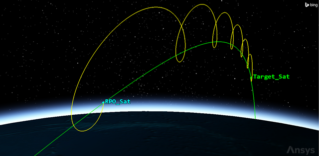
rpo_sat to target_sat
Targeting a maneuver to circumnavigate the target sequence
You've successfully targeted a maneuver to transfer RPO_Sat from its initial position 30 degrees away in True Anomaly from Target_Sat, to a position 1 km away from Target_Sat on Target_Sat's VBar. You now need to compute the maneuver required to initiate the relative orbit to circumnavigate Target_Sat in a stable manner.
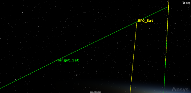
target_Sat to RPO_sat
Inserting a new Target Sequence
Insert a new Target Sequence after the Target Approach sequence.
- Return to RPO_Sat's () Properties ().
- Right-click on the bottom return segment () in the MCS.
- Select Insert Before... in the shortcut menu.
- Select Target Sequence () when the Segment Selection dialog box opens.
- Click to accept your selection and to close the Segment Selection dialog box.
- Rename Target Sequence () to Target NMC.
Inserting a Maneuver segment to represent the burn
You will do a three-axis burn to circumnavigate Target_Sat. Since you will be starting your circumnavigation relative orbit on Target_Sat's VBar, it is primarily a radial maneuver required to formulate the orbit. But there are specific conditions that need to be met in order to achieve the natural motion circumnav, the primary condition being that the orbital periods of RPO_Sat and Target_Sat are matched.
- Right-click on the return segment () below Target_NMC () in the MCS.
- Select Insert Before... in the shortcut menu.
- Select Maneuver () when the Segment Selection dialog box opens.
- Click to accept your selection and to close the Segment Selection dialog box.
Updating the Maneuver segment's properties
Choose a new name and color for the Maneuver segment.
- Select Maneuver () in the MCS.
- Click Segment Properties () in the MCS toolbar.
- Type Burn2 in the Name field when the Edit Segment dialog box opens.
- Open the Color picker drop-down.
- Select white.
- Click to accept your changes and to close the Edit Segment dialog box.
Setting Burn2's Thrust axes
Update Burn2's thrust axes to reference the RIC coordinate frame.
- Select the Attitude tab.
- Open the Attitude Control drop-down list.
- Select Thrust Vector.
- Click the Thrust Axes ellipsis ().
- Open the Filter by drop-down list when the Select Reference dialog box opens.
- Select All Objects.
- Select RPO_Sat () in the object list.
- Select RIC (
 ) in the Axes for: RPO_Sat list.
 - Click to accept your change and to close the Select Reference dialog box.
Setting up the control parameters
Set up the control parameters for the Burn2 Maneuver segment.
- Select the following Cartesian targets ():
X
Y
Z
- Keep the default values for each dimension (0 m/sec).
- Click to accept your changes.
Selecting Burn2's results to achieve relative orbital parameters
You would like to target desired orbital parameters relative to Target_Sat at the end of the Burn2 Maneuver segment.
- Select Burn2 () in the MCS.
- Click .
- Expand () Formation () in the Available Components list when the User - Selected Results - Burn2 dialog box opens.
- Move () Rel Mean SemiMajor Axis () to the Selected Components list.
- Expand () the Relative Motion () in the Available Components list.
- Move () CrossTrackRate () to the Selected Components list.
- Click to accept your selections and to close the User - Selected Results - Burn2 dialog box.
- Click to accept your changes.
Adding this value to the differential corrector will ensure you achieve a relative orbit where the orbital period is matched with Target_Sat's.
Adding this value to the differential corrector will ensure you achieve a relative orbit that is completely in plane with Target_Sat.
Adding a Propagate segment
You want Burn2 to generate the Delta-V that will propagate RPO_Sat to the negative VBar or -Y side of Target_Sat. That is essentially a position where RPO_Sat is crossing the Y-Z plane of Target_Sat, where the Y-Z plane represents the In-Track/Cross-Track plane of Target_Sat in the stopping condition's properties.
- Right-click on Burn2 () in the MCS.
- Select Insert After... in the shortcut menu.
- Select Propagate () when the Segment Selection dialog box opens.
- Click to accept your selection and to close the Segment Selection dialog box.
Updating the Propagate segment's properties
Update the name and color of the Propagate sequence.
- Select the new Propagate () in the MCS.
- Click Segment Properties () in the MCS toolbar.
- Type Prop2PlaneCross in the Name field when the Edit Segment dialog box opens.
- Open the Color picker drop-down.
- Select a color that's different from the other Propagate () segments in the MCS.
- Click to accept your changes and to close the Edit Segment dialog box.
Adding a new stopping condition
Add a Y-Z Plane Cross stopping condition for the Prop2PlaneCross Propagate segment.
- Click New... (
 ) in the Stopping Conditions toolbar.
 - Select Y-Z Plane Cross () when the New Stopping Condition dialog box opens.
- Click to accept your selection and to close the New Stopping Condition dialog box.
- Select Duration in the Stopping Conditions list.
- Click Delete (
 ) in the Stopping Conditions toolbar.
 - Click the Coord. System ellipsis ().
- Select Target_Sat () in the Objects list when the Select Reference dialog box opens.
- Select RIC (
 ) in the Systems for: Target_Sat list.
 - Click to accept your selections and to close the Select Reference dialog box.
Changing the stopping condition's satisfaction criterion
Change the satisfaction criterion for the Y-Z Plane Cross stopping condition to Cross Decreasing. Cross Decreasing means the stopping condition is satisfied when the parameter reaches a value equal to the trip value while decreasing.
- Open the Criterion drop-down list.
- Select Cross Decreasing.
Setting the results
You want to achieve a symmetrical relative position on the negative VBar of Target_Sat from where RPO_Sat is currently located. The satellite is currently 1 km in the positive VBar, so you want to add a relative position component as the result.
- Click .
- Expand () the Relative Motion () in the Available Components list when the User - Selected Results - Prop2PlaneCross dialog box opens.
- Move () InTrack () to the Selected Components list.
- Click to accept your selection and to close the User - Selected Results - Prop2PlaneCross dialog box.
- Click to accept your changes.
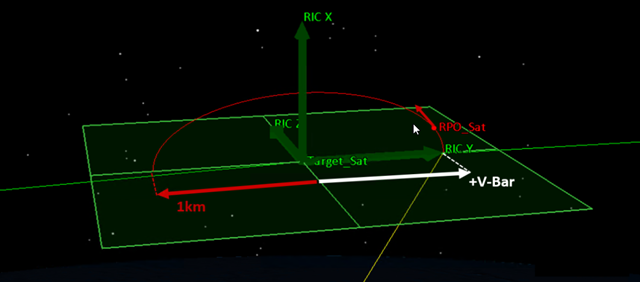
RPO_Sat Propagating to Target YZ Plane Cross
Creating three differential correctors
Similarly to Target Approach, set up Target NMC to walk into a circumnav relative orbit in a stepwise fashion. To do this, use three nested differential correctors.
Building the first differential corrector
In natural motion relative orbits, the radial and in-track components are intrinsically linked. This can easily be determined by the LTT transformation of the Clohessy-Wiltshire equations. For that reason, it makes sense to solve for the relative radial and in-track components in the same differential corrector.
- Select the Target NMC () in the MCS.
- Rename Differential Corrector to Target Radial and InTrack in the Profiles list.
- Click Properties... () in the Profiles toolbar.
Setting the control parameters
You're going to solve for the Radial and InTrack maneuver components for the NMC.
- Select the Variables tab when the Target Radial and InTrack dialog box opens.
- Select Use for ImplsiveMnvr.Pointing.Cartesian.X in the Control Parameters list.
- Enter 0.1 m/sec in the Perturbation field.
- Enter 10 m/sec in the Max. Step field.
- Select Use for ImplsiveMnvr.Pointing.Cartesian.Y in the Control Parameters list.
- Enter 0.1 m/sec in the Perturbation field.
- Enter 10 m/sec in the Max. Step field.
Setting the equality constraints
Since you are varying the Radial and InTrack Delta-V, you need to add the Relative Semimajor Axis and relative InTrack position as equality constraints.
- Select Use for Rel_Mean_Semimajor_Axis.
- Enter 1e-05 km in the Tolerance field.
- Select Use for InTrack.
- Enter -1 km in the Desired Value cell.
- Enter 0.001 km in the Tolerance field.
- Open the Method drop-down list in the Scaling panel.
- Select By tolerance.
This will ensure that the maneuver is computed to place RPO_Sat (![]() ) 1km on the other side of Target_Sat (
) 1km on the other side of Target_Sat (![]() ) when crossing the YZ Plane.
) when crossing the YZ Plane.
Setting the convergence criteria
Specify the convergence criteria and related parameters for the profile.
- Select the Convergence tab.
- Open the Convergence Criteria drop-down list.
- Select Either equality constraints or last control parameter updates within tolerance.
- Click to accept your changes and to close the Target Radial and InTrack dialog box.
Building the second differential corrector
Add a second differential corrector the Target NMC sequence.
- Click Copy () in the Profiles toolbar.
- Click the Paste () in the Profiles toolbar.
- Rename Target Radial and InTrack1 to Target CrossTrackRate.
- Click Properties... () in the Profiles toolbar.
Setting the control parameters
In this differential corrector, you will only solve for the cross-track component of the circumnav ellipse. The LTT equations tell you the cross-track component of natural motion ellipses are decoupled from the radial and in-track components. So, solving for the cross-track component by itself makes sense.
- Select the Variables tab in the Target CossTrackRate dialog box.
- Clear the ImplsiveMnvr.Pointing.Cartesian.X Use check box.
- Clear the ImplsiveMnvr.Pointing.Cartesian.Y Use check box.
- Select Use for ImplsiveMnvr.Pointing.Cartesian.Z in the Control Parameters list.
- Enter 0.1 m/sec in the Perturbation field.
- Enter 10 m/sec in the Max. Step field.
Setting the equality constraints
You are varying the cross-track Delta-V, so you need to add the CrossTrackRate as an equality constraint.
- Clear the Rel_Mean_Semimajor_Axis Use check box.
- Clear the InTrack Use check box.
- Select Use for CrossTrackRate.
- Enter 1e-06 km/sec in the Tolerance field.
- Click to accept your changes and to close the Target CossTrackRate dialog box.
Building the third differential corrector
Build a third differential corrector to target both Radial Intrack and CrossTrack Rate.
- Click New... () in the Profiles toolbar.
- Select Differential Corrector () when the New... dialog box opens.
- Click to accept your selection and to close the New... dialog box.
- Rename Differential Corrector to Target RI and CrossTrack Rate.
- Click Properties... () in the Profiles toolbar.
Setting the control parameters
In this differential corrector, you will use the solutions previously determined for the X, Y, and Z maneuver components and further refine them in a single differential corrector.
- Select Use for ImplsiveMnvr.Pointing.Cartesian.X in the Control Parameters list when the Target RI and CrossTrack Rate dialog box opens.
- Enter 0.1 m/sec in the Perturbation field.
- Enter 10 m/sec in the Max. Step field.
- Select Use for ImplsiveMnvr.Pointing.Cartesian.Y in the Control Parameters list.
- Enter 0.1 m/sec in the Perturbation field.
- Enter 10 m/sec in the Max. Step field.
- Select Use for ImplsiveMnvr.Pointing.Cartesian.Z in the Control Parameters list.
- Enter 0.1 m/sec in the Perturbation field.
- Enter 10 m/sec in the Max. Step field.
Setting the equality constraints
You need to add all three equality constraints for the Rel_Mean_Semimajor_Axis, InTrack and CrossTrack.
- Select Use for CrossTrackRate.
- Enter 1e-06 km/sec in the Tolerance field.
- Select Use for Rel_Mean_Semimajor_Axis.
- Enter 1e-05 km in the Tolerance field.
- Select Use for InTrack.
- Enter -1 km in the Desired Value cell.
- Enter 0.001 km in the Tolerance field.
- Open the Method drop-down list in the Scaling panel.
- Select By tolerance.
Setting the convergence criteria
Specify the convergence criteria and related parameters for the third differential corrector profile.
- Select the Convergence tab.
- Open the Convergence Criteria drop-down list.
- Select Either equality constraints or last control parameter updates within tolerance.
- Click to accept your changes and to close the Target RI and CrossTrack Rate dialog box.
- Click to accept your changes.
Propagating the natural motion circumnav for 12 hours
Add a Propagate segment after the Target NMC Target Sequence.
- Right-click the bottom Return segment () in the MCS.
- Select Insert Before... in the shortcut menu.
- Select Propagate () when the Segment Selection dialog box opens.
- Confirm that the Trip value is 43200 sec (12 hr). This is the default value.
- Click to accept your selection and to close the Segment Selection dialog box.
Setting the Propagate segment's properties
Update the name and color of the Propagate segment.
- Select Propagate1 () in the MCS.
- Click Segment Properties () in the MCS toolbar.
- Type NMC in the Name field when the Edit Segment dialog box opens.
- Open the Color picker drop-down.
- Choose a color that different for the other Propagate () segments in the MCS.
- Click to accept your changes and to close the Edit Segment dialog box.
- Click to accept your changes.
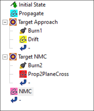
final mcs view
Solving for the control parameters
Update the Target NMC sequence's action and re-run the entire MCS.
- Save () your scenario.
- Select Target NMC () in the MCS.
- Open the Action drop-down list.
- Select Run Active Profiles.
- Click Run Entire Mission Control Sequence () in the MCS toolbar.
- Return to RPO_Sat's () Properties ().
- Click Clear Graphics () in the MCS toolbar.
- Click to accept your changes.
Viewing changes in the 3D Graphics window
View the changes in the 3D Graphics window.
- Bring the 3D Graphics window to the front.
- Zoom to RPO_Sat ().
- Use your mouse to view RPO_Sat () and Target_Sat ().
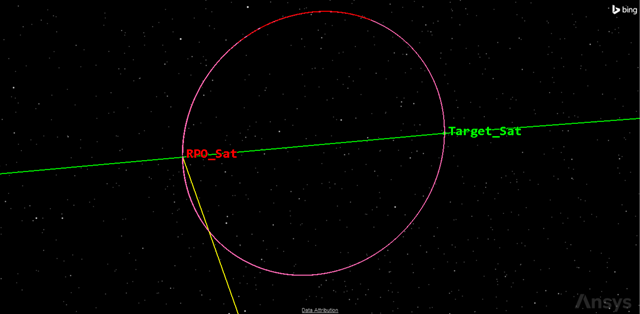
RPO_SAT AND TARGET_SAT
Evaluating the maneuvers performed
Use the information provided by the Target Sequence status window to evaluate the maneuvers performed during the RPO.
Reviewing the data in the Target Sequence status window
Review the results of the Target.NMC.Target RI and CrossTrack Rate Target Sequence.
- Bring the Target.NMC.Target RI and CrossTrack Rate Target Sequence status window to the front.
- Review the data in the New Value column which shows the Delta-V magnitude.
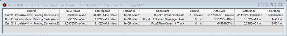
Target.NMC.Target RI and CrossTrack Rate target sequence status window
![]() ). At first glance, the large in-track (Y) maneuver component makes sense. The satellite arrived on Target_Sat's (
). At first glance, the large in-track (Y) maneuver component makes sense. The satellite arrived on Target_Sat's (![]() ) VBar and needed to perform an in-track maneuver to move to the negative VBar. What may not make sense is the larger radial (X) maneuver component. What is the reason for this?
) VBar and needed to perform an in-track maneuver to move to the negative VBar. What may not make sense is the larger radial (X) maneuver component. What is the reason for this?
Generating a summary report in the MCS
Generate a summary report to get a feel for the total Delta-V required for this maneuver.
- Bring RPO_Sats () Properties () to the front.
- Select Burn2 () in the MCS.
- Click Summary (
 ) in the MCS toolbar.
 - In the Summary, note the DeltaV Magnitude (for example, approximately 81 m/sec).
- Close the Summary report.
Generating a Maneuver Summary Report in the Report & Graph Manager
Generate a Maneuver Summary Report to get a better understanding of the RPO maneuver.
- Right-click RPO_Sat () in the Object Browser.
- Select Report & Graph Manager... (
 ) in the shortcut menu.
 - Select Maneuver Summary (
 ) in the Installed Styles () list when the Report & Graph Manager opens.
 - Click .
- Take a moment to evaluate the total Delta-V reported for Burn2 (for example, approximately 81 m/sec).
- Look at the differential corrector results for the first target sequence (Target Approach).
Remember that the resulting magnitude of the maneuver vector is computed using the root of the sum of the squares (RSS). So:

It's worth asking again "why is the radial maneuver required?" What if there were little or no radial component in the maneuver?

The tiny cross-track component wouldn't even register, and you'd be left with just the expected in-track component.
To understand the reason for the radial component, you need to go back to Burn1, the rendezvous maneuver.
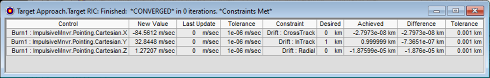
target ric target sequence status window
Notice it too has a large radial component of approximately -84.6 m/sec required to perform the maneuver. Remember, RPO_Sat had the same orbital parameters as Target_Sat, but was offset in True Anomaly by 30 degrees. In many ways, you could say RPO_Sat was "coplanar" with Target_Sat, with matched inclinations and the same altitude. So why was the radial component required?
It goes back to the caveat at the beginning of this lesson. This rendezvous was not optimal.
Understanding the effects of osculating elements and HPOP
You propagated Target_Sat and RPO_Sat in Astrogator using the High Precision Orbit Propagator (HPOP) using osculating elements. What are osculating elements? "Osculating elements are the true time-varying orbital elements, and they include all periodic (long- and short-periodic) and secular effects," notes D. A. Vallado in "Fundamentals of Astrodynamics and Applications," in his chapter on general perturbation techniques. "They represent the high-precision trajectory and are useful for highly accurate simulations."
If you propagated the satellites using a two-body propagator, without osculating elements, the cross-track component would disappear. It just would not have been realistic.
For computing and planning rendezvous using full-force models and osculating elements, choosing optimal departure and arrival times to minimize the differences in orbital periods and other elements is critical. Careful consideration of those times could have minimized the need for much of the radial maneuver component during the rendezvous, and ultimately to maintain the in-track NMC.
Visualizing the osculating elements
Create an RIC Plot for Target_Sat and RPO_Sat.
- Right-click on Target_Sat () in the Object Browser.
- Select Report & Graph Manager... (
 ) in the shortcut menu.
 - Select the RIC (
 ) graph in the Installed Styles list when the Report & Graph Manager opens.
 - Click .
- Select RPO_Sat () in the Available Objects list of the Assigned Object dialog box.
- Click .
- Click to accept your choice and to close the Assigned Object dialog box.
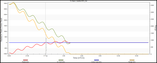
RIC GRAPH
Zooming in for clarity
Zoom in on the RIC plot to see the effects of the initial maneuver.
- Click .
- Enter 1 sec in the Step field.
- Select Enter on your keyboard.
- Using your left mouse button, lasso the cross-range plot line from the beginning of the graph to the point when the rendezvous happens.
- Keep zooming in, keeping yourself centered on 0, until you can see the initial maneuver (Burn1) affect the cross-track component.
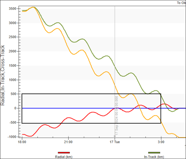
Zoom In box - RIC Graph
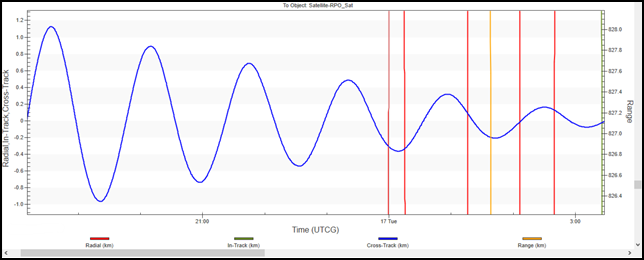
RIC graph zoomed in
Notice the initial drift in cross-track during the 600 sec propagation segment, then the large oscillation that takes place when Burn1 occurs (vertical black line).
The maneuver took place when the relative difference in the cross-track components of Target_Sat and RPO_Sat were not zero. Additionally, you can see that the cross-track component moved by over a kilometer when you initiated the transfer. You needed to raise RPO_Sat's orbit to drift over to Target_Sat, and it turns out that the rate at which Inclination and RAAN vary, are very sensitive to altitude. So during the transfer, the planes of the two satellites were moving differently and at different rates.
Additionally, to minimize the radial components of the maneuvers and the overall Delta-V required, you needed to apply careful consideration of the timing of the maneuvers. You can visualize this by plotting an altitude plot of RPO_Sat.
Creating a custom Altitude graph to view changes
Generate your custom altitude graph to view the changes in RPO_Sat's ephemeris when it enters the transfer to Target_Sat.
Creating a custom graph style
Create a custom graph called Altitude.
- Return to the Report & Graph Manager.
- Select RPO_Sat () in the Object Type list.
- Select My Styles () in the Styles panel.
- Click Create new graph style (
 ) in the Styles toolbar.
 - Enter Altitude for the graph's name.
- Select Enter on your keyboard to open Altitude's (
 ) Properties ().
Choosing a data provider
Choose your data provider, group and element for the graph.
- Expand () Astrogator Values () in the Data Providers list.
- Expand () the Geodetic () group.
- Select the Altitude (
 ) element.
 - Move () Altitude () to the Y Axis list.
- Click to accept your selection and to close the Properties Browser.
Generating the graph
Generate the custom altitude graph.
- Select Altitude () in the My Styles () list.
- Click .
- Close all graphs and the Report & Graph Manager.
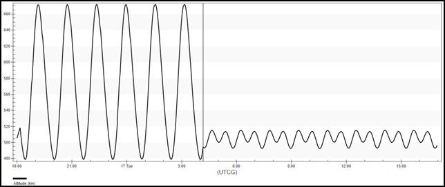
altitude graph
Notice the drastic change in altitude early in RPO_Sat's ephemeris when it enters the transfer to Target_Sat. Also notice the how there is a jog in the altitude as RPO_Sat enters the NMC around Target_Sat.
These redirections manifest as radial components, and are indicative of suboptimal departure and arrival times.
You could implement a more robust solution by incorporating an optimization target profile like the Interior Point Optimizer (IPOPT) or the Sparse Nonlinear Optimizer (SNOPT), to determine the optimal times to initiate the transfer and the drift duration.
Entering near-optimal departure and drift times
To demonstrate the effect of more-optimal departure and arrival times, enter the following propagation times and rerun the MCS.
- Return to RPO_Sat's () Properties ().
- Select Propagate () in the MCS.
- Enter 0 sec in the Trip field.
- Select Drift () in the MCS.
- Enter 34325 sec in the Trip field.
- Click to accept your changes.
- Click Run Entire Mission Control Sequence () in the MCS toolbar.
The first Maneuver Summary report showed a total Delta-V of approximately 172 m/sec. How does the total Delta-V required compare?
Saving your work
Clean up your workspace and save your work.
- Close any open reports, properties and tools.
- Save () your work.
Summary
You followed some basic steps in modeling the mission of one satellite approaching another already in orbit using Astrogator. The two satellites were in the same orbital plane, with the target satellite trailing the mission satellite in True Anomaly. You targeted two in-plane burns to approach and subsequently circumnavigate the target satellite. You created a Mission Control Sequence (MCS) to perform a non-optimal transfer to the target satellite and a maneuver to enter into a Natural Motion Circumnavigation (NMC) relative orbit.
On your own
Try a further step of incorporating a minimum Delta-V Lambert solution into Astrogator via the scripting interface to seed an optimal two-body transfer solution. This will greatly increase the efficiency of the transfer and proximity operations maneuvers. Though not necessary, this "semi-analytic" approach of combining analytic solutions from Lambert with the numerical solutions of Astrogator's search profiles, can be quite successful.