STK Premium (Air) or STK Enterprise
You can obtain the necessary licenses for this tutorial by contacting AGI Support at support@agi.com or 1-800-924-7244.
Required Capability Install: This lesson requires an additional capability installation for STK Terrain Integrated Rough Earth Model (TIREM). The TIREM install is included in the STK Pro software download, but requires a separate install process. Read the Readme.htm found in the STK install folder for installation instructions. You can obtain the necessary install by visiting http://support.agi.com/downloads or calling AGI support.
This lesson requires an internet connection and version 12.9 of the STK software or newer to complete in its entirety. If you have an earlier version of the STK software, you can complete a legacy version of this lesson.
The results of the tutorial may vary depending on the user settings and data enabled (online operations, terrain server, dynamic Earth data, etc.). It is acceptable to have different results.
Capabilities covered
This lesson covers the following capabilities of the Ansys Systems Tool Kit® (STK®) digital mission engineering software:
- STK Pro
- Communications
- Aviator
- Terrain Integrated Rough Earth Model (TIREM)
Problem statement
Engineers and technicians require tools to create simulations and analyze results to plan future missions before spending time and money fielding assets to perform on-site analysis. You are simulating a future training mission where a light aircraft will fly a search pattern over mountainous terrain. You need to determine how well the aircraft receives GPS transmissions. Although illegal to purchase and use in the United States, GPS jammers pose a threat to your test. You want to know how these jammers could affect your communications so you can confidently plan future missions when there is a possibility of GPS interference in the rescue area of operations. A team of engineers will drive to an area centrally located under the aircraft's search pattern to determine if one of these devices will affect the aircraft's reception of the GPS signal.
Solution
Use the STK Pro software and a local, analytical terrain file to design the mountainous training area where the test will take place. Use the Communications capability to build the satellite GPS transmitters, the aircraft's GPS receiver, and measure interference against the GPS signal. Then, use the Aviator capability to create a search pattern for a light aircraft built to specifications. Then, use the Terrain Integrated Rough Earth Model (TIREM) capability to predict radio frequency propagation loss over irregular terrain. Combine these models to understand how the jammer will affect communications in your scenario.
What you will learn
Upon completion of this tutorial, you will be able to:
- Design GPS satellite transmitters, which use GPS Global Antenna Patterns
- Design a GPS receiver, which uses a GPS Fixed Reception Pattern Antenna (FRPA)
- Use radio frequency environmental models and system noise temperature calculations
- Use the Aviator capability to design a simple search pattern for a small aircraft
- Determine GPS reception in the target area
- Create a small GPS interference source
- Use the TIREM capability to predict radio frequency propagation loss over irregular terrain
- Analyze GPS jamming
Creating a new scenario
First, you must create a new STK scenario, then build from there.
- Launch the STK application (
 ).
). - Click
 Create a Scenario in the Welcome to STK dialog box.
 - Enter the following in the STK: New Scenario Wizard:
- Click when you finish
- Click Save (
 ) when the scenario loads.
 - Verify the scenario name and location in the Save As dialog box.
- Click .
| Option | Value |
|---|---|
| Name | GPS_Analysis |
| Location | Default |
| Start | Default date, use 19:00:00.000 UTCG |
| Stop | + 4 hrs |
The STK software automatically creates a folder with the same name as your scenario for you.
Save (![]() ) often during this tutorial!
) often during this tutorial!
Disabling streaming terrain
You're using a local terrain file for analysis. Turn off Terrain Server.
- Right-click on GPS_Analysis () in the Object Browser.
- Select Properties (
 ) in the shortcut menu.
 - Select the Basic - Terrain page when the Properties Browser opens.
- Clear the Use terrain server for analysis check box in the Terrain Server panel.
- Click to confirm your changes and to keep the Properties Browser open.
Modeling the scenario's RF environment
A number of environmental factors can affect the performance of a communications link. Since you're modeling the downlink portion of a satellite transmission, you'll enable rain and atmospheric absorption models at the scenario level. The scenario's
- Select the RF - Environment page.
- Select the Rain, Cloud & Fog tab.
- Select the Use check box in the Rain Model panel.
- Confirm you are using the default
- Select the Atmospheric Absorption tab.
- Select the Use check box.
- Confirm you are using the default
- Click to confirm your selections and to close the Properties Browser.
When enabled, the STK software uses the rain model to estimate the amount of degradation (or fading) of the signal when passing through rain.
Adding analytical and visual terrain
An STK terrain inlay (.pdtt) file can be used both for analysis and for visualization in the 3D Graphics window. Use a preinstalled terrain inlay file to your scenario using the
- Bring the 3D Graphics window to the front.
- Click Globe Manager (
 ) on the 3D Graphics window's Globe Manager toolbar.
 - Click Add Terrain/Imagery (
 ) on the Globe Manager Hierarchy toolbar when Globe Manager opens.
 - Select Add Terrain/Imagery... (
 ) in the drop-down menu.
 - Click the Path ellipsis (
 ) when the Globe Manager: Open Terrain and Imagery Data dialog box opens.
 - Browse to the install directory at C:\Program Files\STK_ODTK 13\Data\Resources\stktraining\imagery when the Browse For Folder dialog box opens.
- Click to confirm your selection and to close the Browse For Folder dialog box.
- Select the StHelens_Training.pdtt check box.
- Click .
- Click when prompted to use StHelens_Training.pdtt for analysis.
Viewing the inlaid terrain
View the terrain inlay in the 3D Graphics window.
- Bring the 3D Graphics window to the front.
- Right-click on StHelens_Training.pdtt (
 ) in the Globe Manager hierarchy.
 - Select Zoom To (
 ) in the shortcut menu.
 - Use your mouse to move around and zoom in and out to view the terrain in the 3D Graphics window.
Inserting operational GPS satellites
Add the currently operational GPS satellites into your scenario.
Using the Standard Object Database
Use the
- Return to the STK application.
- Bring the Insert STK Objects tool (
 ) to the front.
 - Select Satellite (
 ) in the Select An Object To Be Inserted list.
 - Select From Standard Object Database (
 ) in the Select A Method list.
 - Click .
Inserting the operational GPS satellites
Search for operational GPS satellites using the AGI Standard Object Data Service.
- Clear the Data Sources - Local check box.
- Enter GPS in the Name or ID field.
- Scroll down in the Data Sources panel and locate Operational Status.
- Open the Operational Status drop-down list.
- Select Operational.
- Click .
- Select all the satellites in the Results list.
- Click .
- When all the GPS satellites have propagated, click to close the Search Standard Object Data dialog box.
Modeling the GPS satellite transmitters
The STK software's Communications capability simulates the performance of communications systems in the context of their missions. Use the Communicationto model the physical components of your communications system. Start by attaching and modeling the GPS satellites' transmitters.
Inserting a Transmitter object
Attach a
- Bring the Insert STK Objects tool () to the front.
- Insert a Transmitter (
 ) object using the Insert Default () method.
 - Select the first Satellite () object when the Select Object dialog box opens.
- Click to confirm your selection and to close the Select Object dialog box.
- Right-click on Transmitter1 () in the Object Browser.
- Select Rename in the shortcut menu.
- Rename Transmitter1 () GPS_Tx1.
Modeling a GPS satellite transmitter
Use a GPS Satellite Transmitter model with the Transmitter object. This model lets you set up multiple antenna beams, each with its own specs and its own polarization and orientation properties. For this lesson, you are configuring one beam.
- Open GPS_Tx1's () Properties ().
- Select the Basic - Definition page when the Properties Browser opens.
- Click the Transmitter Model Component Selector ().
- Select GPS Satellite Transmitter Model (
 ) when the Select Component dialog box opens.
 - Click to confirm your selection and to close the Select Component dialog box.
Modifying the beam specs
Modify the power parameter of your beam.
- Select the Beams tab.
- Select the Beam Specs sub-tab.
- Enter 27.45 W in the Power field.
- Click to confirm your changes and to keep the Properties Browser open.
Modeling the GPS global antenna pattern
Modify the antenna parameters for your beam. For this analysis, you will use the GPS global antenna pattern. This antenna type models a GPS satellite antenna operating a global beam on the L1, L2 , or L5 frequency bands and uses a polar coordinate system. You will keep things simple, and model the Block IIR, L1 antenna type.
- Select the Antenna sub-tab.
- Select the Antenna sub-tab's Model Specs sub-tab.
- Ensure GPS Global is selected in the Antenna Model field.
- Open the Block Type drop-down list.
- Select IIR, L1.
- Enter 80 % in the Efficiency field.
- Click to confirm your changes and to keep the Properties Browser open.
If you look in the Block Type list, you can see antenna types for the other block types.
Setting right-hand circular polarization
- Select the Antenna sub-tab's Polarization sub-tab.
- Select the Use check box.
- Open the Linear drop-down list.
- Select Right-hand Circular.
- Click to confirm your selection and to keep the Properties Browser open.
Setting the data rate
The transmitter's data rate is a compound dimension with data bits and time as simple dimensions. For public use, the GPS design uses a Coarse/Acquisition pseudo-random noise (PRN) code transmitted at a data rate of 1.023 megabits per second.
- Select the transmitter's Model Specs tab.
- Enter 1.023 Mb/sec in the Data Rate field.
- Click to confirm your change and to keep the Properties Browser open.
Modeling the modulator
The STK software's Communications capability allows you to select from multiple modulators, including user-defined modulators. The GPS Coarse/Acquisition code uses the binary Phase-shift keying (BPSK) modulation technique, which is the default setting. You will also use the Power Spectral Density (PSD) option. The Power Spectral Density option allows the scenario to model the actual spectral shape of the transmitted signal based on the modulation, data rate, etc. PSD is used to determine the Bandwidth Overlap Factor. By using signal PSD, you combine the entire signal including losses in your analysis. The nulls are where the main lobe and side lobes drop to zero.
- Select the Modulator tab.
- Select the Use Signal PSD check box.
- Enter 1 in the Number of Spectrum Nulls field.
- Click to confirm your changes and to keep the Properties Browser open.
Notice that setting the number of spectrum null to 1 automatically sets the Bandwidth to 2.046 MHz, which you can see in the Signal Bandwidth panel.
Visualizing the antenna pattern
The Transmitter's object's
- Select the 3D Graphics – Attributes page.
- Select the Show Volume check box in the Volume Graphics panel.
- Click to confirm your selection and to keep the Properties Browser open.
- Bring the 3D Graphics window to the front.
- Right-click on the Satellite () object to which you attached the Transmitter () object in the Object Browser.
- Select Zoom To in the shortcut menu.
- Return to GPS_Tx1's () Properties () when finished.
- Clear the Show Volume check box in the Volume Graphics panel.
- Click to confirm your change and to close the Properties Browser.
![]()
GPS Transmitter Antenna Pattern
Blue shows the maximum gain and red shows the minimum gain.
Reusing the GPS transmitter
- Select GPS_Tx1 () in the Object Browser.
- Click Copy (
 ) on the Object Browser toolbar.
 - Select the next Satellite () object in the Object Browser.
- Click Paste (
 ) on the Object Browser toolbar.
 - Using this method, Paste () the transmitter to the remaining GPS satellites.
You only have to copy the transmitter the first time, then paste it onto the remaining satellites. To save time, you can use the Ctrl+C and Ctrl+V keyboard shortcuts to copy and paste your transmitters to the satellites.
Although there is no need to rename the new transmitters in this tutorial (you can just keep the STK numbering), this is one instance where in a real world scenario, matching transmitter names to the satellite can help you when running a report or graph.
Modeling the test area
Use an Area Target object to outline the test area. An Area Target object models a region on the surface of a central body. Using an Area Target object will also simplify creating a flight route for the test aircraft.
Inserting an Area Target object
Insert an Area Target object using the
- Bring the Insert STK Objects tool () to the front.
- Insert an Area Target (
 ) object using the Area Target Wizard (
 ) method.
 - Enter Test_Area in the Name field when the Area Target Wizard opens.
- Click four times.
- Set the following in the Points panel in the order shown:
- Click to confirm your changes and to close the Area Target Wizard.
| Latitude | Longitude |
|---|---|
| 46.00 deg | -123.00 deg |
| 46.00 deg | -122.00 deg |
| 47.00 deg | -122.00 deg |
| 47.00 deg | -123.00 deg |
Making the area target visible
Earlier in the scenario, you turned off streaming terrain. This affects the view of the Area Target object when using a local terrain file. You need to change your Scenario object's 3D Graphics Global Attributes so you can view the Area Target on the terrain.
- Open GPS_Analysis' () Properties ().
- Select the 3D Graphics - Global Attributes page when the Properties Browser opens.
- Open the On Terrain drop-down list in the Surface Lines panel.
- Select On.
- Click to confirm your selection and to close the Properties Browser.
Decluttering labels
Objects located on the surface of the terrain could be covered by the terrain, which makes them unreadable. You can fix this by making a change to the
- Bring the 3D Graphics window to the front.
- Click Properties () on the 3D Window Defaults toolbar.
- Select the Details page when the Properties Browser opens.
- Select the Enable check box in the Label Declutter panel.
- Click to confirm your selection and to close the Properties Browser.
Viewing the test area
View Test_Area in the 3D Graphics window.
- Bring the 3D Graphics window to the front.
- Zoom to Test_Area ().
- Zoom out on the 3D Graphics window to view the entire outline of Test_Area.
- Use your mouse to zoom back to the surface and explore the terrain.
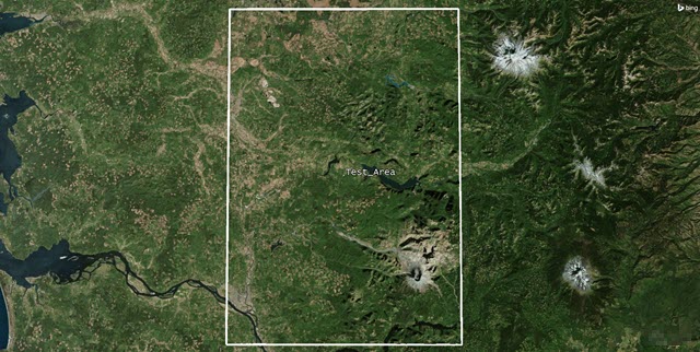
test area
Look at the southeastern corner of the test area. This is Mount St. Helens.
Modeling the test aircraft
Your test will use a light aircraft equipped with a GPS receiver to fly search pattern inside of the designated test area. Use the Aviator capability to model the aircraft and its flight path. The Aviator capability models the aircraft's route through a sequence of curves parameterized by well-known performance characteristics of aircraft, including cruise airspeed, climb rate, roll rate, and bank angle.
Inserting an Aircraft object
Insert an
- Bring the Insert STK Objects tool () to the front.
- Insert an Aircraft (
 ) object using the Insert Default () method.
 - Rename Aircraft1 () Test_Acft.
Using the Aviator propagator
Select the Aviator propagator to create the test aircraft's flight route.
- Open Test_Acft's () Properties ().
- Select the Basic - Route page when the Properties Browser opens.
- Open the Propagator drop-down list.
- Select Aviator.
- Click to confirm your selection and to keep the Properties Browser open.
- Click when the Flight Path Warning dialog box opens.
- Read the information in the Flight Path Warning dialog box.
- Click to close the Flight Path Warning dialog box.
Selecting the aircraft model
In Aviator, an
- Click Select Aircraft (
 ) in the Initial Aircraft Setup toolbar.
 - Select Basic General Aviation (
 ) in the User Aircraft Models (
 ) list in the Select Aircraft dialog box.
 - Click to confirm your selection and to close the Select Aircraft dialog box.
- Click to confirm your changes and to keep the Properties Browser open.
Note that Basic General Aviation (![]() ) is read only (
) is read only (![]() ). Read-only items in the Aviator Catalog Manager cannot be modified. They can be duplicated and then modified when needed.
). Read-only items in the Aviator Catalog Manager cannot be modified. They can be duplicated and then modified when needed.
Inserting the first procedure
Every mission must have at least one
- Right-click on Phase 1 (
 ) in the Mission List.
 - Select Insert First Procedure for Phase ... (
 ) in the shortcut menu.
Selecting the site type
Each phase is composed sites and procedures. A
- Select STK Area Target () in the Select Site Type list in the Site Properties dialog box.
- Select Test_Area () in the Link To list.
- Click .
Selecting the procedure type
A
- Select AreaTargetSearch () in the Select Procedure Type list when the Procedure Properties dialog box opens.
- Clear the Use Aircraft Default Cruise Altitude check box in the Altitude panel.
- Enter 8000 ft in the Altitude field.
- Set the following in the Search Options panel:
- Enter 5.00 in the Turn Factor field, located in the Enroute Options panel.
- Click to confirm your selections and to close the Procedure Properties dialog box.
- Click to confirm your changes and to close the Properties Browser.
| Option | Value |
|---|---|
| Max Separation | 5 nm |
| Course Mode | Override |
| Centroid True Course | 90 deg |
The Turn Factor is the maximum amount — expressed as a multiplier — that the turn radius will be increased to minimize the bank angle required to complete the turn.
Viewing the aircraft's flight route
View Test_Acft's flight route in the 3D Graphics window.
- Bring the 3D Graphics window to the front.
- Zoom to Test_Area ().
- Zoom in or out using your mouse so that you can see Test_Acft's flight route.
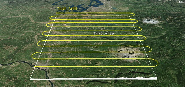
Aircraft Flight Route
Aviator calculated a search pattern based on the parameters that you set. The course is defined based on Test_Area's centroid.
Modeling the GPS receiver
The test aircraft is equipped with a GPS receiver, which uses a Fixed Reception Pattern Antenna (FRPA).
Inserting a Receiver object
Insert and attach a
- Bring the Insert STK Objects tool () to the front.
- Insert a Receiver (
 ) object using the Insert Default () method.
 - Select Test_Acft () when the Select Object dialog box opens.
- Click to confirm your selection and to close the Select Object dialog box.
- Rename Receiver1 () GPS_Rx.
Using a Complex Receiver model
A Complex Receiver model enables you to select among a variety of analytical and realistic antenna models and to define the characteristics of the selected antenna type.
- Open GPS_Rx's () Properties ().
- Select the Basic - Definition page when the Properties Browser opens.
- Click the Receiver Model Component Selector ().
- Select Complex Receiver Model () when the Select Component dialog box opens.
- Click to confirm your selection and to close the Select Component dialog box.
Setting the amplifier model specs
Adjust the low noise amplifier (LNA) losses and gain. A low noise amplifier is an electronic amplifier that amplifies a very low-power signal without significantly degrading its signal-to-noise ratio.
- Select the Model Specs tab.
- Set the following:
- Click to confirm your changes and to keep the Properties Browser open.
| Option | Value |
|---|---|
| Antenna to LNA Line Loss | 1 dB |
| LNA Gain | 20 dB |
| LNA to Receiver Line Loss | 10 dB |
Modeling a GPS FRPA antenna pattern
The receiver requires a
- Select the Antenna tab.
- Select the Model Specs sub-tab.
- Click the Antenna Model Component Selector ().
- Select GPS FRPA () when the Select Component dialog box opens.
- Click to confirm your selection and to close the Select Component dialog box.
- Click to confirm your changes and to keep the Properties Browser open.
Modeling linear polarization
The receiver is linearly polarized with the electrical field aligned with the reference axis. Although it would be optimal for the receiver's antenna polarization to match the transmitter's, it is common to transmit with circular polarization but receive using linear polarization. You will lose power due to the polarization mismatch which will be modeled.
- Select the Polarization sub-tab.
- Select the Use check box.
- Ensure the Polarization is set to Linear, which is the default selection.
- Set the Cross-Pol Leakage Threshold to -30 dB.
- Click to confirm your changes and to keep the Properties Browser open.
You only use Cross-Pol Leakage with a Receiver object. Whenever the STK software detects a complete polarization mismatch between the transmitted signal and the received signal under ideal conditions, the cross polarization leakage value is applied to model the less-than-ideal real-world performance.
Setting the antenna's orientation
The STK software provides
- Select the Orientation sub-tab.
- Enter -90 deg in the Elevation field.
- Click to confirm your change and to keep the Properties Browser open.
Modeling system noise temperature
The Receiver's System Noise Temperature allows you to specify the system's inherent noise characteristics. These can help simulate real-world RF situations more accurately.
- Select the System Noise Temperature tab.
- Select the Compute option.
- Enter 4.8 dB in the Noise Figure field in the LNA panel.
- Select the Compute option in the Antenna Noise panel.
- Select the following check boxes:
- Earth
- Sun
- Atmosphere
- Rain
- Cosmic Background
- Click to confirm your changes and to keep the Properties Browser open.
Using a Terrain Mask constraint
The test aircraft is flying over a mountainous area, and you'll need to account for any line-of-sight access blockages between the GPS satellite transmitters and the aircraft-mounted GPS receiver. Since are using analytical terrain, you can add a Terrain Mask constraint to the Receiver object to model the terrain blockages.
- Select the Constraints - Active page.
- Click Add new constraints (
 ) in the Active Constraints toolbar.
 - Type terrain in the Search field in the Select Constraints to Add dialog box.
- Select Terrain Mask in the Constraint Name list.
- Click .
- Click to close the Select Constraints to Add dialog box.
- Click to confirm your selection and to keep the Properties Browser open.
Visualizing the antenna pattern
Set the volume graphics and view the antenna pattern in the 3D Graphics window.
- Select the 3D Graphics - Attributes page.
- Select the Show Volume check box in the Volume Graphics panel.
- Click to confirm your selection and to keep the Properties Browser open.
- Bring the 3D Graphics window to the front.
- Zoom to Test_Acft ().
- Return to GPS_Rx's () Properties () when finished.
- Clear the Show Volume check box in the Volume Graphics panel.
- Click to confirm your changes and to close the Properties Browser.

Receiver Antenna Pattern
Determining GPS reception quality
Determine the signal quality between the GPS transmitters and the GPS receiver. A link budget reports the values that determine the GPS reception. For the purposes of this scenario, you will focus on one column in the link budget: C/No (dB * Hz). The carrier to noise density ratio (C/No) where C is the carrier power and No is equal to kT (Boltzmann's constant × system temperature) is the noise density. It is equivalent to C/N with a normalized Bandwidth (B=1). In this instance, the compound dimension being used is Spectral Density and the Base Dimension is Bandwidth × Ratio. The Bandwidth is in Hertz (Hz).
Computing access
Before you can generate a link budget, you must first compute the accesses between the aircraft-mounted GPS receiver and the GPS satellite transmitters using the
- Right-click on GPS_Rx () in the Object Browser.
- Select Access... (
 ) in the shortcut menu.
 - Select all of the Satellite () objects in the associated objects list when the Access tool opens.
- Right-click on one of the Satellite () objects.
- Select Expand All in the shortcut menu.
- Right-click on one of the Transmitter () object.
- Select Select All Transmitters in the shortcut menu.
- Click
 .
.
Be patient. This could take a couple of minutes.
Creating a link budget report
Generate a
- Click .
- Select all of the Access (
 ) objects in the Object Type list when the Report & Graph Manager opens.
 - Select the Specify Time Properties option in the Time Properties panel.
- Set the following time property options:
- Select the Link Budget - Detailed (
 ) report in the Installed Styles (
 ) folder in the Styles list.
 - Click .
| Option | Value |
|---|---|
| Use step size / time bound | Selected |
| Step size: | 60 sec |
Reviewing the Link Budget - Detailed report
Review the report. How is the reception between your GPS receiver and the satellite transmitters based on C/No (dB*Hz) of greater than or equal to 35? Keep in mind you're going to see fluctuations due to RF environment, location of the satellites (overhead, low on the horizon), distance, etc. Any fields in the report where it says "Data Unavailable" means there was no access between the GPS receiver and the GPS transmitter on that satellite.
- Browse to the C/No (dB * Hz) column.
- Scroll down through the report.
- View other data based on settings:
- Atmos Loss (dB)
- Rain Loss (dB)
- Tatmos (K)
- Train (K)
- Tsun (K)
- Tearth (K)
- Tcosmic (K)
- Tantenna (K)
- Close the Link Budget - Detailed report, the Report & Graph Manager, and the Access tool.
Modeling the test team's location
The test team is deploying a small, portable GPS jammer near the center of the test area.
Inserting a Place object
Insert a
- Bring the Insert STK Objects tool () to the front.
- Insert a Place (
 ) object using the Insert Default () method.
 - Rename Place1 () Test_Team.
Setting test team's location
The test team is deployed in a clearing at the end of a dirt road, very near the test area's centroid. Their jammer will be placed atop a 2-meter antenna.
- Open Test_Team's () Properties ().
- Select the Basic - Position page when the Properties Browser opens.
- Set the following in the Position panel:
- Click to confirm your changes and to close the Properties Browser.
| Option | Value |
|---|---|
| Latitude | 46.4995 deg |
| Longitude | -122.4944 deg |
| Height Above Ground | 2 m |
Height Above Ground raises the Test_Team Place object two meters above the surface of the terrain. When you attach a Transmitter object to Test_Team, the Transmitter object's antenna will also be raised two meters above the terrain's surface.
Viewing the test team's location
View the test team's location in the 3D Graphics window. This is where the GPS jammer will be deployed. Look at its location compared to the test aircraft's flight route.
- Bring the 3D Graphics window to the front.
- Zoom to Test_Team ().
- Use your mouse to view the area where the GPS jammer will be deployed and its location relative to the test aircraft.
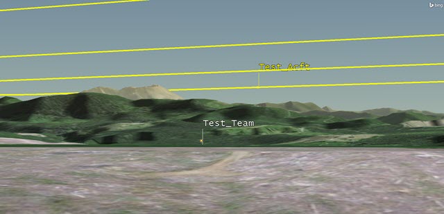
Test Team and Aircraft
Determining the range from the test team to the test aircraft
The jammer's manufacturer claims its maximum effective radius is 400 meters. Determine how far the test aircraft will be from test team during the test using an
- Right-click on Test_Team () in the Object Browser.
- Select Access... (
 ) in the shortcut menu.
 - Select Test_Acft () in the Associated Objects list when the Access tool opens.
- Click .
- Click in the Reports panel.
- Scroll down to the Statistics at the bottom of the AER report.
- Note the minimum and maximum range of the Test_Acft () from Test_Team ().
- Close (
 ) the AER report when finished.
 - Click to close the Access tool.
The aircraft never gets closer than approximately one to two kilometers from the test team. This is well outside the manufacturer's claimed radius of 400 meters.
Modeling the portable jammer
Model the test team's jammer with a new Transmitter object.
Attaching a Transmitter object to Test_Team
Attach a Transmitter object to Test_Team.
- Bring the Insert STK Objects tool () to the front.
- Insert a Transmitter () object using the Insert Default () method.
- Select Test_Team () when the Select Object dialog box opens.
- Click to confirm your selection and to close the Select Object dialog box.
- Rename Transmitter2 () Jammer.
Configuring the GPS jammer
Use a Complex Transmitter Model for the jammer.
- Open Jammer’s () Properties ().
- Select the Basic - Definition page when the Properties Browser opens.
- Click the Transmitter Model Component Selector ().
- Select Complex Transmitter Model () in the Transmitter Models List in the Select Component dialog box.
- Click to confirm your selection and to close the Select Component dialog box.
Setting the model specs
Model the jammer's frequency and power. Most small, portable GPS jammers have similar specifications.
- Select the Model Specs tab.
- Set the following options:
- Click to confirm your changes and to keep the Properties Browser open.
| Option | Value |
|---|---|
| Frequency | 1.57542 GHz |
| Power | 35 W |
Modeling a dipole antenna pattern
For this analysis, you will use a dipole antenna pattern. Dipole antennas are modeled analytically using modeling equations that can be found in standard antenna texts.
- Select the Antenna tab.
- Select the Model Specs sub-tab.
- Click the Antenna Model Component Selector ().
- Select Dipole () when the Select Component dialog box opens.
- Click to confirm your selection and to close the Select Component dialog box.
- Set the following options:
- Click to confirm your changes and to keep the Properties Browser open.
| Option | Value |
|---|---|
| Design Frequency | 1.57542 GHz |
| Length | 7 in |
| Efficiency | 80 % |
Modeling vertical polarization
Set the antenna's polarization to vertical.
- Select the Polarization sub-tab.
- Select the Use check box.
- Open the Linear drop-down list.
- Select Vertical.
- Click to confirm your changes and to keep the Properties Browser open.
Modeling the jammer's modulation
Model the jammer's modulator. The Narrowband Uniform analytical modulator models narrowband jammers.
- Select the Modulator tab.
- Open the Name drop-down list.
- Select Narrowband Uniform.
- Click to confirm your selection and to keep the Properties Browser open.
Preparing the jammer's transmitter for TIREM
Disable the Line-of-sight, Terrain Mask, and Az-El Mask constraints to take advantage of the over-the-horizon analysis functionality of TIREM.
- Select the Constraints - Active page.
- Clear the Enable check box for Line Of Sight in the Active Constraints list.
- Click to confirm your change and to keep the Properties Browser open.
Using the TIREM capability
Recall that you enabled both rain and atmospheric absorption models at the scenario level to predict your link budget between the GPS satellites' transmitters and the aircraft's GPS receiver. The jamming device needs to take into account how terrain will affect its performance. The Terrain Integrated Rough Earth Model capability adds fidelity to the calculation and dynamic modeling of point-to-point line-of-sight effects for link performance in communications. It does this by taking into account the effect of irregular terrain and non-line-of-sight effects. The maximum height for these models is 30 km. You can set this RF Environment setting at the object level.
- Select the RF - Environment page.
- Select the Atmospheric Absorption Tab.
- Select the Use check box.
- Click the Atmospheric Absorption Model Component Selector ().
- Select the newest TIREM () component when the Select Component dialog box opens.
- Click to confirm your selection and to close the Select Component dialog box.
- Click to confirm your changes and to close the Properties Browser.
Adding receiver interference sources
You can add interference sources to a GPS receiver's properties. Then, you can assess their impact on the performance of the receiver.
- Open GPS_Rx's () Properties ().
- Select the Basic - Definition page.
- Select the Interference tab.
- Select the Use check box.
- Select Test_Team/Jammer () in the Available Emitters list.
- Move (
 ) Test_Team/Jammer () to the Assigned Emitters list.
 - Click to confirm your selection and to close the Properties Browser.
Your link budgets will be automatically recomputed. Be patient. This can take a couple of minutes.
Checking for interference
You can check for interference using a pre-built report.
Generating a Link Budget - Interference report
Generate a
- Right-click on GPS_Rx () in the Object Browser.
- Select Report & Graph Manager... (
 ) in the shortcut menu.
 - Open the Object Type drop-down list in the Report & Graph Manager.
- Select Access.
- Select all of the Access () objects in the Object Type list, except Place-Test_Team-To-Aircraft-Test_Acft ().
- Select the Specify Time Properties option in the Time Properties panel.
- Set the following time properties options:
- Select the Link Budget - Interference () report in the Installed Styles folder () in the Styles list.
- Click .
| Option | Value |
|---|---|
| Use step size / time bound | Selected |
| Step size | 60 sec |
Reviewing the report
Review the report to identify the extent of the interference.
- Scroll to the right and locate the C/No (dB*Hz) and C/(No+Io) (dB*Hz) columns in your generated report.
- Scroll down through the report to see how the portable jamming transmitter is affecting the aircraft's GPS reception.
The C/(No+Io) (dB*Hz) column measures interference. This is the carrier to noise-plus-interference density ratio (C/(No+Io)), where C is the carrier power, No is kT (Boltzmann's constant × system temperature), and Io is the interference power spectral density.
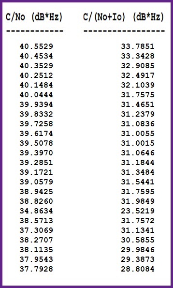
Column One: No Interference / Column Two: Interference
Scrolling through the report, you can see that the jammer is definitely affecting GPS reception, despite the manufacturer's claims.
Saving your work
Clean up and close out your scenario.
- Close any open reports, properties, and the Report & Graph Manager.
- Save () your work.
Summary
This tutorial demonstrated a link budget that focused on a specific value: C/No (dB * Hz). Representational averages were used for both rain and atmospheric absorption losses. GPS Transmitters and the aircraft's GPS receiver were built to model authentic civilian hardware. When the C/No (dB * Hz) value was equal to or greater than 35, GPS reception was good. Actual web specifications for illegal hand-held GPS jammers lead consumers to think they have a very limited jam radius. The jammer specifications used in this scenario stated that the jammer had a jamming radius of up to 400 meters. As you can see, the jammer reached out much further than that when targeting C/No (dB * Hz). You can verify this by matching Access range times against successful interference periods (C/No (dB*Hz) versus C/(No+Io) (dB*Hz)). You also took into account the effect terrain had on the jammer using TIREM.This tutorial is an excellent example of applying real-world hardware specifications and environmental factors into an STK scenario to obtain a better understanding of what the engineering team should expect to see during an actual test.
On your own
You can use this setup to perform additional analyses:
- Match the Antenna Type to the different GPS block types, and rerun the link budget analysis.
- Match the receiver's polarization to the transmitter's polarization, and rerun the link budget analysis.
- Place two or three jammers in different locations through the test area, and analyze interference.
- Place a jammer on the aircraft and a GPS receiver on the ground, and analyze interference.