STK Pro, STK Premium (Air), STK Premium (Space), or STK Enterprise
You can obtain the necessary licenses for this tutorial by contacting AGI Support at support@agi.com or 1-800-924-7244.
Required product install:installation of the Navigation Files Plugin, which is included with
The results of the tutorial may vary depending on the user settings and data enabled (online operations, terrain server, dynamic Earth data, etc.). It is acceptable to have different results.
This tutorial requires an Internet connection or the ability to transfer files from an Internet connected computer to a computer not connected to the Internet. The files will be downloaded from the United States Coast Guard Navigation Center.
Capabilities covered
This lesson covers the following capabilities of the Ansys Systems Tool Kit® (STK®) digital mission engineering software:
- STK Pro
- Coverage
Problem statement
You are testing a new radar system that is designed to provide highly accurate location information for aircraft flying through the United States' airspace. To determine the fidelity of the new radar system, you want to compare an aircraft's Global Positioning System (GPS)-determined location information to the radar tracking information. You will be making a test flight, during which you will be monitoring the aircraft's location via GPS. To accurately test the radar system, you need to simulate the GPS position navigation accuracy (PACC) over the contiguous United States and determine the Horizontal Dilution of Precision (HDOP) along the aircraft's flight route. Your test will take place today.
Solution
Use the Navigation Files Plugin to model the current GPS satellite constellation and the Coverage capability to determine PACC at the planned flight altitude of 20,000 feet over the contiguous United States during a 24-hour period. Next, measure the GPS HDOP at altitude over the route of the test flight, which will fly from Long Beach, California to Philadelphia, Pennsylvania.
What you will learn
Upon completion of this tutorial, you will understand the following:
- How to download and use GPS almanac files in your analysis
- How to download and use satellite outage files in your analysis
- How to download and use prediction support files in your analyses
- How to measure only the accuracy associated with the positional portion of the navigation solution
- How to use the Coverage tool to perform single-object coverage analysis
- How to measure the dilution of precision for the horizontal (latitude / longitude) components of the positional portion of the navigation solution
Video guidance
Watch the following video. Then follow the steps below, which incorporate the systems and missions you work on (sample inputs provided).
Creating a new scenario
First, you must create a new scenario, and then build from there.
- Launch the STK application (
 ).
). - Click
 Create a Scenario when the Welcome to STK dialog box opens.
 - Enter the following in the STK: New Scenario Wizard:
- Click to confirm your changes, close the STK: New Scenario Wizard and load your scenario.
- Click Save (
 ) when the scenario loads.
 - Verify the scenario name and location in the Save As dialog box.
- Click .
| Option | Value |
|---|---|
| Name | PACC_HDOP |
| Start | Today |
| Stop | + 1 day |
The STK application automatically creates a folder with the same name as your scenario for you.
Save (![]() ) often during this scenario!
) often during this scenario!
Turning off streaming terrain
By default, the STK application connects to the Ansys Geospatial Data Cloud to distribute Earth terrain data for analysis and visualization. Turn off
- Right-click on PACC_HDOP () in the Object Browser.
- Select Properties (
 ) in the shortcut menu.
 - Select the Basic - Terrain page when the Properties Browser opens.
- Clear the Use terrain server for analysis check box in the Terrain Server panel.
- Click to confirm your change and to close the Properties Browser.
Preparing the 2D Graphics window for situational awareness
Before you begin to define your analysis area, clear all the
- Bring the 2D Graphics window to the front.
- Click Properties () in the 2D Window Defaults toolbar.
- Select the Imagery page when the Properties Browser opens.
- Clear the Show check box in the Background Image panel.
- Click to confirm your change and to close the Properties Browser.
Defining the analysis area
Use an
- Bring the Insert STK Objects (
 ) tool to the front.
 - Select Area Target (
 ) in the Select An Object To Be Inserted list.
 - Choose Select Countries and US States (
 ) in the Select A Method list.
 - Click .
- Select United_States_of_America in the list of pre-built Area Target objects when the Select Countries and US States dialog box opens.
- Ensure the Primary Area Only option is selected in the Insert panel.
- Click .
- Click to close the Select Countries and US States dialog box.
Selecting Primary Areas Only during the creation process will ensure that only the contiguous United States is outlined. If you had selected All Areas, an area target representing each of the Hawaiian islands, Alaska and all its islands, etc. would have been imported.
Viewing the contiguous United States in the 2D Graphics window
Use the Zoom In function in the 2D Graphics window to outline the contiguous United States.
- Click Zoom In (
 ) in the 2D Window Defaults toolbar.
 - Using your left mouse button, draw a box around the contiguous United States.
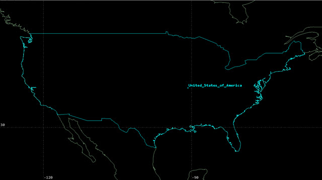
2D View of the contiguous United States
Viewing the contiguous United States in the 3D Graphics window
Use the Zoom In function in the 3D Graphics window to outline the contiguous United States.
- Bring the 3D Graphics window to the front.
- Click and grab to turn the Earth until you can see the contiguous United States.
- Click Zoom In () in the 3D Window Defaults toolbar.
- Using your left mouse button, draw a box around the contiguous United States.
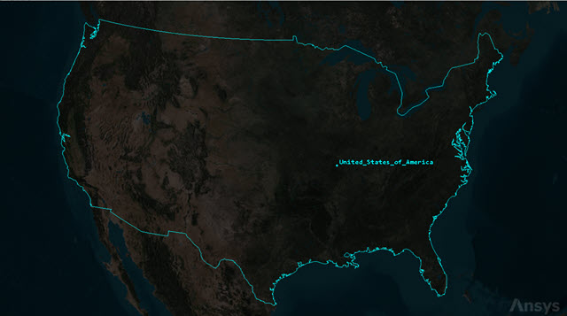
3D View of the contiguous United States
Clearing the Area Target's label
You don't need to display the Area Target's United_States_of_America label or the visible centroid. Clear those options by updating its
- Open United_States_of_America's () Properties ().
- Select the 2D Graphics - Attributes page when the Properties Browser opens.
- Clear the following check boxes in the Inheritable Settings panel:
- Inherit from Scenario
- Show Label
- Show Centroid
- Click to confirm your changes and to close the Properties Browser.
Downloading the current satellite almanac file to propagate the GPS satellites
The GPS almanac is a set of data that every GPS satellite transmits, and it includes information about the state (health) of the entire GPS satellite constellation and coarse data on every satellite's orbit. The U.S. Coast Guard makes GPS almanacs in the System Effectiveness Model (SEM) format available on a routine basis — currently once per day. SEM almanac files are ASCII messages containing the almanac information and usually have a .al3 file extension. Note that the Coast Guard almanac data includes only ephemeris and clock data, and does not include covariance or the high-accuracy GPS to UTC time correlation.
- Open your preferred web browser.
- Navigate to the U.S. Coast Guard's Navigation Center's GPS NANUS, Almanacs, OPS Advisories, & SOF page at
- Scroll down to the Almanacs (YUMA & SEM) section.
- Click the Current SEM Almanac - .al3 link to download the most recent almanac file, current_sem.al3.
- Keep your web browser open.
Copying the almanac file to your scenario folder
Copy the downloaded almanac file to your scenario folder.
- Go to the location of your downloaded SEM almanac in Windows File Explorer.
- Right-click on current_sem.al3.
- Select Copy in the shortcut menu.
- Select Documents in the navigation pane.
- Navigate to your scenario folder (for example, C:\Users\<username>\Documents\STK_ODTK 13\PACC_HDOP).
- Right-click in the content pane.
- Select Paste in the shortcut menu.
If you chose a non-default folder in which to store your scenarios during the STK application install, you will need to place the current_sem.al3 file in your custom location.
Downloading the current satellite outage file
Satellite outage files (SOFs) provide information about GPS satellite outages. Taking these outages into account is crucial for obtaining an accurate navigation error prediction. Without considering outages, your navigation errors may be smaller than actually observed. The U.S. Space Force produces a new SOF each time a new outage is completed, experienced or predicted. You can download the current SOF from U.S. Coast Guard Navigation Center. The SOF provides GPS outage information for historical, current and predicted outages.
- Return to the GPS NANUS, Almanacs, OPS Advisories, & SOF page at
- Scroll down to the Satellite Outage File (SOF) section.
- Click the Current SOF - .sof link to download the most recent SOF file, current_sof.sof.
- Keep your web browser open.
Copying the outage file to your scenario folder
Copy the SOF to your scenario folder.
- Navigate to the location of the downloaded current_sof.sof file in Windows File Explorer.
- Copy current_sof.sof.
- Select Documents in the navigation pane.
- Navigate to your scenario folder (for example, C:\Users\<username>\Documents\STK_ODTK 13\PACC_HDOP).
- Paste current_sof.sof in your scenario folder.
- Keep Windows File Explorer open.
If you chose a non-default folder in which to store your scenarios during the STK application install, you will need to place the current_sof.sof file in your custom location.
Inserting the GPS Constellation
Use the From GPS Almanac method to insert the GPS constellation from the almanac file you downloaded from the U.S. Coast Guard.
Inserting a new Satellite object
Insert the GPS constellation by inserting a Satellite object.
- Bring the Insert STK Objects tool () to the front.
- Insert a Satellite (
 ) object using the From GPS Almanac (
 ) method.
Using the From GPS Almanac method
The
- Select the Automatic - File method in the Catalog Source panel when the Insert From GPS Almanac dialog box opens.
- Click the ellipsis (
 ) next to the File field.
 - Navigate to your scenario folder (for example, C:\Users\<username>\Documents\STK_ODTK 13\PACC_HDOP) when the Select GPS Almanac File dialog box opens.
- Select current_sem_al3.
- Click to confirm your selection and to close the Select GPS Almanac File dialog box.
- Click .
- Select the Create Constellation from Selected Satellites check box in the Constellation panel.
- Enter GPSConstellation in the Name field.
- Click to insert the current GPS satellites and to create the GPS Constellation.
- Click to close the Insert From GPS Almanac dialog box.
This option will direct STK to reload the specified almanac file every time the satellite is propagated. When you load that scenario, it will repropagate the satellites based on the date. You will however need to ensure you update your almanac file accordingly when you reopen your scenario in the future.
All GPS satellites found in the almanac will appear on the left of the Insert from GPS Almanac dialog box.
Clearing GPS satellites' orbit tracks
You don't need to visualize the orbits and ground tracks of the GPS constellation's satellites. Clear them by batch updating their 2D Graphics attributes.
- Multi-select all of the Satellite () objects in the Object Browser.
- Click Properties () on the Object Browser toolbar.
- Select the 2D Graphics - Attributes page when the Properties Browser opens.
- Clear the Inherit from Scenario check box in the Inheritable Settings panel.
- Clear the Show Orbit check box.
- Clear the Show Ground Track check box.
- Click to confirm your changes and to close the Properties Browser.
Loading the SOF into the GPS Satellite Outage tool
Use the GPS Satellite Outage tool to use the GPS satellite outage information from the SOF in your analysis.
- Select the View menu.
- Select Toolbars.
- Select Navigation Files Support in the Toolbars submenu.
- Select GPSConstellation (
 ) in the Object Browser.
 - Click Add GPS Satellite Outages (
 ) on the Navigation Files Support toolbar.
 - Increase the size of the Add GPS Satellite Outages window when it opens, if needed, to see the full extent of the tool.
- Click the ellipsis () in the Select GPS Satellite Outage Data panel.
- In the Open dialog box, browse to the location of the SOF file (for example, C:\Users\<username>\Documents\STK_ODTK 13\PACC_HDOP).
- Select current_sof.sof.
- Click .
This will display the Navigation Files Support toolbar ( ).
).
A message noting "Satellite Outage Data Loaded" will appear on the bottom of the Select GPS Satellite Outage Data panel.
Applying the outages to the GPS Constellation
With your SOF file loaded, apply the outage to the GPS constellation.
- Ensure GPSConstellation is selected in the Apply to Which GPS Constellation? list.
- Click .
- Read the message that satellite outage data has been updated in the Update Complete dialog box.
- Click to close the message.
- Review the outage information in the Outage Results Applied panel.
- Click to close the GPS Satellite Outage tool.
The outages for your scenario are determined by your scenario's time frame. Once applied, the text box at the bottom of the tool will list any outages for your scenario.
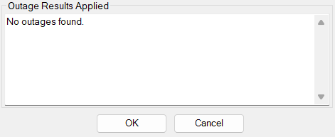
No GPS Outages
If an outage is found, the tool will list the interval of the outage. The identification of the object is based on the PRN assigned to it, which is matched to the space vehicle identifier (SVID) value in the SOF.
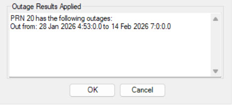
GPS Outage found
If an outage is reported, the STK application will remove the satellite from your analysis by creating a temporal constraint. You can open the satellite's properties and go to the Constraints - Active page. An Intervals constraint will already exist in the Active Constraints list. In the Interval Constraint's Constraint Properties list, the outage interval from the SOF will automatically be loaded.
Defining the coverage area
The STK software's Coverage capability enables you to analyze the global or regional coverage provided by one or more assets (e.g. vehicles, facilities, sensors) while considering all access constraints. You want to assess coverage of the contiguous United States based on the boundaries of the area target that is being used to outline that area. You will need to specify the region being examined (United_States_of_America), how each grid point should be treated, and what assets will be used to examine the region (GPSConstellation).
Inserting a Coverage Definition object
The first thing you need to do is define the coverage area using a
- Bring the Insert STK Objects () tool to the front.
- Insert a Coverage Definition object (
 ) using the Insert Default () method.
 - Right-click on CoverageDefinition1 () in the Object Browser.
- Select Rename in the shortcut menu.
- Rename CoverageDefinition1 () ContUS_Cov.
Choosing the Grid Area of Interest
Coverage analyses are based on the accessibility of assets (objects that provide coverage) and geographical areas. For analysis purposes, you can further refine the geographical areas of interest using regions and points. Points have specific geographical locations, and the STK application uses them in the computation of asset availability. Regions are closed boundaries that contain points. The STK application computes accessibility to a region based on accessibility to the points within that region. The combination of the geographical area, the regions within that area, and the points within each region is called the coverage grid.
- Right-click on ContUS_Cov () in the Object Browser.
- Select Properties () in the shortcut menu.
- Select the Basic - Grid page when the Properties Browser opens.
- Open the Type drop-down list in the Grid Area of Interest panel.
- Select Custom Regions.
- Open the Area Of Interest drop-down list.
- Select Area Targets.
- Select United_States_of_America () in the Area Targets list.
- Move (
 ) United_States_of_America () to the Selected Regions list.
Defining the point granularity and altitude
The statistical data computed during a coverage analysis is based on a set of locations, or points, which span the specified grid area of interest. You can determine the spacing between grid points using the Grid Definition options. For this simulation, you will analyze navigation accuracy every one degree at an altitude of 20,000 feet.
- Enter 1 deg in the Lat/Lon field in the Grid Definition - Point Granularity panel.
- Enter 20000 ft in the Altitude above WGS84 field in the Point Altitude panel.
- Click to confirm your changes and to keep the Properties Browser open.
Assigning the coverage assets
The Coverage Definition Assets properties enable you to
- Select the Basic - Assets page.
- Select GPSConstellation () in the Assets list.
- Click .
- Click to confirm your selection and to keep the Properties Browser open.
Turning off the automatic re-computation of accesses
The STK application automatically recomputes accesses every time you update an object on which the coverage definition depends (such as an asset). If you want control as to when the STK application computes coverage, you can turn this off The Coverage Definition's object's
- Select the Basic - Advanced page.
- Clear the Automatically Recompute Accesses check box in the Access panel.
- Click to confirm your selection and to keep the Properties Browser open.
Raising the grid points visually in the 3D Graphics window
You can visualize the grid points and coverage at 20,000 feet in the 3D Graphics window by updating the Coverage Definition object's
- Select the 3D Graphics - Attributes page.
- Select the Show at Altitude check box in the Fill Options panel.
- Click to accept your changes and to close the Properties Browser.
Viewing the coverage grid in the 2D and 3D Graphics windows
Place the 2D and 3D Graphics windows side-by-side.
- Select the Window menu in the Menu Bar.
- Select Tile Vertically in the Window menu.
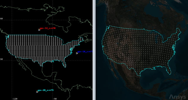
coverage grid in the 2D and 3D graphics windows
Using the Compute Accesses tool
The ultimate goal of coverage is to analyze accesses to an area by using assigned assets and applying necessary limitations upon those accesses. Compute coverage with the Compute Accesses tool.
- Select ContUS_Cov () in the Object Browser.
- Select the CoverageDefinition menu in the Menu Bar.
- Select Compute Accesses in CoverageDefinition menu.
Improving the view in the 2D and 3D Graphics windows
Clear the grid points from the 2D and 3D Graphics windows. This is purely aesthetic and isn't required for analysis.
- Open ContUS_Cov's () Properties ().
- Select the 2D Graphics - Attributes page when the Properties Browser opens.
- Clear the Show Points check box in the Grid panel.
- Click to confirm your change and to close the Properties Browser.
Measuring the accuracy of a navigation solution with a Figure of Merit
You can evaluate navigation accuracy by attaching a Figure of Merit object to the Coverage Definition object of interest. The Navigation Accuracy Figure of Merit type considers the effect of the number of measurements (of those satellites visible at each moment in time), the geometry of the transmitters, and the uncertainty in the one-way range measurements in the computation of the uncertainty in the navigation solution. The uncertainty in the one-way range measurements may be specified as a constant value or as a function of the elevation angle on a transmitter basis.
Inserting a Figure of Merit object
Attach a Figure of Merit object to the ContUS_Cov Coverage Definition object.
- Bring the Insert STK Objects () tool to the front.
- Insert a Figure Of Merit (
 ) object using the Insert Default () method.
 - Select ContUS_Cov () when the Select Object dialog box opens.
- Click to confirm your selection and to close the Select Object dialog box.
- Rename FigureOfMerit1 () PACC.
Selecting a definition type
Select Navigation Accuracy as the definition type.
- Open PACC's () Properties ().
- Select the Basic - Definition page when the Properties Browser opens.
- Open the Type drop-down list.
- Select Navigation Accuracy.
Choosing a static definition of navigation accuracy
You need to set the
- Open the Compute drop-down list.
- Select Maximum.
This will compute maximum uncertainty at each point over the entire coverage interval.
Selecting a specific navigation accuracy measure
Navigation accuracy can be calculated in a
- Open the Method drop-down list.
- Select PACC.
Choosing the allowed number of assets
Although four satellites are needed for the navigation solution, additional satellites can be used to improve the accuracy of the solution.
- Open the Type drop-down list to view the various options.
- Leave the default type of Over Determined.
The Over Determined option computes the navigation accuracy based on all of the currently available assets. If you select this method, you need to involve a minimum of three assets in the navigation solution.
Specifying a time step
In the Time Step field, enter the value to be used during the sampling of the dynamic definition for use in the static definition.
- Enter 60 sec in the Time Step field.
- Click to confirm your changes and to close the Properties Browser.
Checking asset range uncertainty
The GPS constellation experiences errors in its ephemeris (position in space) and clock data that translate into positioning errors in GPS receivers. Knowing these uncertainties helps provide a better prediction of the aircraft's GPS receiver's accuracy.
Downloading the current Prediction Support File
Using prediction support files (PSFs), you can model your navigation accuracy with higher fidelity. PSFs provide statistical error data for both GPS ephemeris and satellite clock errors. You can download the current PSF from the AGI website.
- Return to your web browser.
- Navigate to https://data.agi.com/pub/Catalog/PSF.
- Click the Current.psf link to download the most recent PSF.
- Close your web browser.
- Navigate to the location of the downloaded Current.psf file in Windows File Explorer.
- Copy Current.psf.
- Select Documents in the navigation pane.
- Navigate to your scenario folder (for example, C:\Users\<username>\Documents\STK_ODTK 13\PACC_HDOP).
- Paste Current.psf in your scenario folder.
- Close Windows File Explorer.
If you chose a non-default folder in which to store your scenarios during the STK application install, you will need to place the Current.psf file in your custom location.
Opening the Navigation Files Plugin
Use the
- Select PACC () in the Object Browser.
- Click Add Navigation Uncertainties (
 ) on the Navigation Files Support toolbar.
Using the Navigation Files Plugin
Load the PSF file into your scenario.
- Increase the size of the Add Navigation Uncertainties window when it opens.
- Click the ellipsis () in the GPS Satellites panel.
- Navigate to your Scenario folder (for example, C:\Users\<username>\Documents\STK_ODTK 13\PACC_HDOP).
- Select Current.psf.
- Click .
- Ensure the ContUS_Cov/PACC check box is selected in the Apply to Which Navigation FOMs? panel.
- Click .
- Click to confirm and to close the Asset Anomalies dialog box, if necessary.
- Click to close Update Complete dialog box.
- Click to close the Add Navigation Uncertainties window.
Note that a message reading "Uncertainty Data Loaded" has appeared in the GPS Satellites panel.
If there are satellites with reported outages, a An Asset Anomalies message appears, noting that "Assets with these PRNS are not in the PSF File and have not been updated."
A message in the Update Complete dialog box reading "Satellite and receiver uncertainties have been updated." will be displayed.
Viewing the updated uncertainties
The STK application has the ability to use this data on the Navigation Accuracy Figure of Merit properties page. View the updated uncertainties that you applied to your figure of merit.
- Open PACC 's () Properties ().
- Select the Basic - Definition page when the Properties Browser opens.
- Click in the Definition Panel.
- Look in the Asset Range Uncertainty panel in the Figure of Merit NA Uncertainties Model dialog box.
- Look in the Receiver Range Uncertainty panel.
- Click to close the Figure of Merit NA Uncertainties Model dialog box.
Notice the constant value for each satellite has been updated with values from the PSF file.
These values have likewise been adjusted.
Generating a Grid Stats Over Time report
You want to visualize the quality of coverage in the 2D and 3D Graphics windows. To accurately display contour levels for figures of merit in the 2D and 3D Graphics windows, you should know the approximate range of values for the current Figure Of Merit. You can use the Report & Graph Manager for the Figure Of Merit to identify the widest range of values that were computed. Generate a Grid Stats Over Time report, which summarizes the minimum, maximum, and average of the figure of merit's dynamic value over the entire grid as a function of time.
- Right-click on PACC () in the Object Browser.
- Select Report & Graph Manager... (
 ) in the shortcut menu.
 - Select the Grid Stats Over Time (
 ) report in the Installed Styles (
 ) folder of the Styles panel when the Report & Graph Manager opens.
 - Click .
- Scroll through the report to see the data.
- Close the report when you are finished viewing it.
To set up the contour levels, you need to identify the smallest value from the Min column and the largest value from the Max column. There is an easier way to do this rather than scrolling.
Creating a custom report
You can modify the contents and format of an existing report style by changing its
- Return to the Report & Graph Manager ().
- Select the Grid Stats Over Time () report in the Installed Styles () folder of the Styles panel.
- Click Duplicate Style (
 ) on the Styles toolbar.
Adding Summary Options
Set up the Summary Options to include the minimum and maximum value outputs. The min and max values are found after doing an iterative search using the report values as an initial sample set and then sub-sampling for the global min and max. The values are found to within a time tolerance of 5 msec.
- Select the Content page when the Properties Browser opens.
- Select Overall Value by Time-Minimum in the Report Contents list.
- Click .
- Select the Min check box in the Summary Options - Statistics panel when the Options dialog box opens.
- Click to confirm your selection and to close the Options dialog box.
- Select Overall Value by Time-Maximum in the Report Contents list.
- Click .
- Select the Max check box in the Summary Options - Statistics panel when the Options dialog box opens.
- Click to confirm you selection and to close the Options dialog box.
- Click to confirm your changes and to close the Properties Browser.
Renaming and generating the custom report
Although it's not required, it's a good idea to rename your custom report.
- Right-click on Grid Stats Over Time (
 ) in the My Styles () folder in the Styles panel.
 - Select Rename in the shortcut menu.
- Rename Grid Stats Over Time () Custom Grid Stats Over Time.
- Click .
Viewing and understanding the data
The report gives you a lot of data. For now, you are interested in the minimum and maximum values for your 24-hour analysis period. Recall that a standard applied by the U.S. Government is less than or equal to 2.0 meters.
- Scroll to Statistics at the bottom of the report.
- Take note of the minimum - minimum (best value) and maximum - maximum (worst value) values which you will use to create contours in the 2D and 3D Graphics windows.
- Close the Custom Grid Stats Over Time report.
- Click to close the Report & Graph Manager.
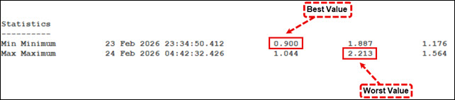
minimum and maximum values
Creating dynamic contours
You can control the display of coverage results with contour graphics depicting the various levels of coverage provided by the assigned assets over time. Display the quality of coverage based on the scenario time by using dynamic contours by updating the
- Return to PACC's () Properties ().
- Select the 2D Graphics - Animation page.
- Enter 25 in the % Translucency field in the Show Points As panel.
Defining the contour levels and colors
Define the contour levels and colors.
- Select the Show Contours option in the Display Metric panel.
- Click the in the Level Attributes panel.
- Enter the following values in the Level Adding panel:
- Click .
- Enter the following values in the Level Attributes panel:
- Select the Natural Neighbor option in the Contour Interpolation (points must be filled) panel.
- Click to confirm your changes and to keep the Properties Browser open.
| Option | Value |
|---|---|
| Add Method | Start, Stop, Step |
| Start | Statistics - Min Minimum value (for example, 0.900 m) |
| Stop | Statistics - Max Maximum value (for example, 2.213 m) |
| Step | 0.2 m |
| Option | Value |
|---|---|
| Color Method | Color Ramp |
| Start Color | Blue (best value) |
| End Color | Red (worst value) |
STK will interpolate the value of the Figure Of Merit for each screen pixel within the coverage area. It will use a natural neighbor algorithm based on the computed values of the Figure Of Merit at the grid points. If the Figure of Merit is discrete, STK will round interpolated values to the nearest integer.
Displaying the Contour Legends
Insert a legend display in the 2D and 3D Graphics windows.
- Click in the Level Attributes panel.
- Click when the Animation Legend for PACC window opens.
- Select the Show at Pixel Location check box in the 2D Graphics Window panel when the Figure of Merit Legend Layout dialog box opens.
- Select the Show at Pixel Location check box in the 3D Graphics Window panel.
- Enter Navigation Accuracy (Meters) in the Title field in the Text Options panel.
- Enter 2 in the Number Of Decimal Digits field.
- Enter 50 in the Color Square Width (pixels) field in the Range Color Options panel.
- Click to confirm your changes and to close the Figure of Merit Legend Layout dialog box.
- Close the Animation Legend for PACC window.
- Click to close the Properties Browser.
Viewing the contours in the 2D Graphics window
You've set your color ramp such that blue will represent a low PACC (which is preferable) and red will represent a high PACC.
- Bring the 2D Graphics window to the front.
- Click Start (
 ) in the animation toolbar to animate the scenario.
 - Click Reset (
 ) when finished.
 - Clear the check box next to PACC () in the Object Browser to remove the graphics.
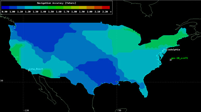
Dynamic contours for position Navigation accuracy
Your contours will look different from the above image.
Building the test flight
The mission aircraft is flying from Long Beach, California, to Philadelphia, Pennsylvania. You can use Place objects as waypoints for the mission.
Inserting the first waypoint for the mission aircraft
Insert a Place object to represent Long Beach.
- Bring the Insert STK Objects () tool to the front.
- Insert a Place (
 ) object using the From City Database (
 ) method.
 - Enter Long Beach in the Name field when the Search Standard Object Data dialog box opens.
- Click .
- Select Long Beach - California in the Results list.
- Click .
Inserting the second waypoint
Insert a second Place object to represent Philadelphia.
- Enter Philadelphia in the Name field.
- Click .
- Select Philadelphia - Pennsylvania in the Results list.
- Click .
- Click to close the Search Standard Object Data dialog box.
Inserting an Aircraft object
An
- Go to the Insert STK Objects () tool.
- Insert an Aircraft (
 ) object using the Insert Default () method.
 - Rename Aircraft1 () Test_Flight.
Defining Test_Flight's flight route
Use the Great Arc propagator to create the flight route from Long Beach to Philadelphia.
- Open Test_Flight's () Properties ().
- Select the Basic - Route page when the Properties Browser opens.
- Look in the Propagator field. GreatArc is the default propagator.
- Bring the 2D Graphics window to the front.
- Click Maximize (
 ) in the upper right corner of the 2D Graphics window.
 - Click on the Long_Beach marker ().
- Click on the Philadelphia marker ().
- Return to Test_Flight's () Properties ().
This will make it easier to see the entirety of the route.
Be careful! Each click on the 2D Graphics window is recognized and added as an aircraft route waypoint.
Changing the waypoint altitude
You want to analyze Test_Flight at an altitude of 20,000 feet
- Click .
- Select the Altitude check box when the Set All Grid Values dialog box opens.
- Enter 20000 ft in the Altitude field.
- Click to confirm your change and to close the Set All Grid Values dialog box.
- Click to confirm your changes and to close the Properties Browser.
Viewing the flight route in the 2D and 3D Graphics windows
You can view Test_Flight's route in the 2D and 3D Graphics windows.
- Click Restore the window to normal size (
 ) in the upper right corner of the 2D Graphics window.
 - Click Start () in the Animation toolbar to animate the scenario.
- Click Reset () when finished.
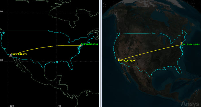
Flight route in the 2D and 3D graphics windows
Measuring HDOP with single-object coverage
Use the single-object coverage method to determine coverage if you are interested in coverage of a small number of well-defined locations or along the trajectory of a moving object. The main differences between normal and single-object coverage are:
- You can use single-object coverage to analyze objects with time-dependent positions
- You can only analyze one figure of merit at a time using single-object coverage
Perform a single-object coverage analysis on the aircraft to determine the Horizontal Dilution of Precision (HDOP) along the flight route from Long Beach to Philadelphia. HDOP is very important in aviation. HDOP measures the quality of GPS positioning along the horizontal plane. This ensures proper spacing between aircraft at the same altitude.
Currently, the Navigation Files Plugin cannot be used with single-object coverage.
Defining single-object coverage
Start by opening the Coverage tool.
- Right-click on Test_Flight () in the Object Browser.
- Select Coverage... (
 ) in the shortcut menu.
Assigning assets to a single object
To determine coverage for a single object, you must assign one or several assets for use in coverage computations. The STK application uses assets to calculate whether coverage to the object is possible. If you define a figure of merit for the coverage, the STK application measures coverage to the object from the assets by the figure of merit values.
- Select GPSConstellation () in the Assets list when the Coverage tool opens.
- Click .
- Click .
Defining a DOP Figure Of Merit
- Click in the Figure of Merit panel.
- Set the following options when the Specify Figure of Merit dialog box opens:
- Click to confirm your changes and to close the Specify Figure of Merit dialog box.
- Note of the number in the Value field. This is the maximum HDOP value along Test_Flight's route.
- Click to confirm your changes and to keep the Coverage tool open.
| Option | Value |
|---|---|
| Type | Dilution Of Precision |
| Compute | Maximum |
| Method | HDOP |
| Type | Over Determined |
| Time Step | 60 sec |
Graphing the HDOP FOM value
Creating a
- Click in the Graphs panel.
- View the data in the graph.
- Place your cursor on the smallest value in the graph.
- Take note of the minimum value out to the hundredth and round down (for example, if your value is 0.64, use 0.63).
- Place your cursor on the largest value in the graph.
- Take note of the maximum value out to the hundredth and round up (for example, if your value is 0.87, use 0.88).
- Close the FOM Value graph.
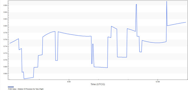
HDOP fom value graph
Your graph will be different from the image shown above. In the above image, the HDOP values all fall below a value of 2, which indicates excellent accuracy.
You will use these values to create color contours along Test_Flight's route.
Creating the contour graphics
Visualize the quality of coverage as Test_Flight flies from Long Beach to Philadelphia.
- Return to the Coverage tool ().
- Click in the Graphics panel.
- Click in the Level Attributes panel when the Contours... dialog box opens.
- Enter the following in the Level Adding panel:
- Click .
- Enter the following values in the Level Attributes panel:
- Click to confirm your changes and to keep the Contours... dialog box open.
| Option | Value |
|---|---|
| Start | Rounded-down minimum FOM graph value |
| Stop | Rounded-up maximum FOM graph value |
| Step | 0.05 |
| Option | Value |
|---|---|
| Use Color Ramp | Selected |
| Select ramp colors | Blue in the first field, Red in the second field |
| Line Width | Thickest |
Displaying the Legend window
Insert a legend display in the 2D and 3D Graphics windows.
- Click .
- Click when the Static Legend for ObjectFOM window opens.
- Select the Show at Pixel Location check box in the 2D Graphics Window panel when the Figure of Merit Legend Layout dialog box opens.
- Select the Show at Pixel Location check box in the 3D Graphics Window panel.
- Enter HDOP in the Title field in the Text Options panel.
- Enter 2 in the Number Of Decimal Digits field.
- Enter 50 in the Color Square Width (pixels) field in the Range Color Options panel.
- Click to confirm your changes and to close the Figure of Merit Legend Layout dialog box.
- Close the Static Legend for ObjectFOM window.
Viewing the flight route in the 2D Graphics window
Close out your open tools so can view the flight route in the 2D Graphics window.
- Click to close the Contours... dialog box.
- Click to close the Coverage tool.
- Bring the 2D Graphics window to the front.
- Click Start () in the Animation toolbar to animate the scenario.
- Click Reset () when finished.
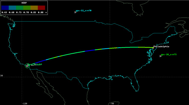
2d graphics window flight route contours
Your contour colors will be different from the above image.
As Test_Flight travels along its path, its label color will also reflect the navigational accuracy at that point in time.
Saving your work
Clean up your workspace and save your work.
- Close any open reports, properties and tools.
- Save () your work.
Summary
This tutorial showed you how to determine GPS position accuracy (PACC) over the contiguous United States and horizontal dilution of precision (HDOP) along a single flight route. You downloaded the current SEM Almanac and satellite outage files from the US Coast Guard Navigation Center. You inserted the GPS constellation from the almanac file. Using the Navigation Files plugin and the GPS Satellite Outage tool, you determined any GPS outages and applied them to your analysis. Using an Area Target object to outline the contiguous United States, you determined PACC at an altitude of 20,000 feet. Next, you created an Aircraft object ,which flew from Long Beach to Philadelphia at an altitude of 20,000 feet. Using the coverage tool, you determined HDOP along the flight route.