STK Premium (Space) or STK Enterprise
You can obtain the necessary licenses for this tutorial by contacting AGI Support at support@agi.com or 1-800-924-7244.
Optional Product Install: This lesson uses the Ansys Electronics Desktop (AEDT)™ electronics systems design platform. You can obtain a license for this product by contacting AGI Support at support@agi.com or 1-800-924-7244.
This lesson requires STK 13.0 or newer to complete in its entirety. If you have an earlier version of the STK software, you can view a legacy version of this lesson.
The results of the tutorial may vary depending on the user settings and data enabled (online operations, terrain server, dynamic Earth data, etc.). It is acceptable to have different results.
For this lesson, you will work with Far Field Data (FFD) files (*.ffd) only. The STK software does not support the use of Near Field Data files (*.nfd).
Capabilities covered
This lesson covers the following capabilities of the Ansys Systems Tool Kit® (STK®) digital mission engineering software:
- STK Pro
- Communications
Problem statement
Engineers and operators want to design a mission to characterize the steam, ash, and lava emissions of active volcanoes in the United States. The objective of the satellite, STKSat, is to image these volcanoes to provide early indications of volcanic eruption and to transmit the images to a ground site for analysis. They want optimize the design of the communications system to ensure the strength of the communications link between the satellite and the ground site allows data to be transmitted and received successfully. The mission requirements for the communication system are as follows:
- The satellite shall downlink health and imagery data at an ultra-high frequency (UHF) of around 435 MHz.
- The satellite shall receive uplink data from the ground site at a very-high frequency (VHF) of around 145 MHz.
- The satellite shall operate with a link margin greater than or equal to 3 dB for imagery and health data to be considered acceptable.
- The satellite shall communicate with a bit error rate of less than or equal to 1e-03 for imagery and health data to be considered acceptable.
Solution
Use the STK software's Communications capability to model a complete RF link between the example mission ground site in Exton, PA and the STKSat spacecraft. You will compare properties such as power and modulators to optimize the RF link, establish a link and telemetry budget for the STKSat mission and analyze the impact of environmental losses on the RF link. Finally, you will vary parameters to optimize the link for the mission requirements.
What you will learn
Upon completion of this tutorial, you will be able to:
- Use the Communications capability to model an RF communications link between a spacecraft and a ground site in real-world conditions
- Import custom-generated antenna pattern files into the STK software and use them analytically
- Analyze the effects of various design parameters on a communications link to optimize the design of a communications system
Video guidance
Watch the following video. Then follow the steps below, which incorporate the systems and missions you work on (sample inputs provided).
Using the starter scenario
The starter scenario contains the constellation of volcanoes to be studied, the imaging satellite and its camera, a Chain object for analysis, and a ground site, which you developed in the
Downloading the starter VDF
Download the zipped starter VDF file.
- Download the zipped folder here: https://support.agi.com/download?type=training&dir=sdf/help&file=CommDesignStarter_v13.zip
- Navigate to the downloaded folder.
- Right-click on CommDesignStarter_v13.zip.
- Select Extract All... in the shortcut menu.
- Set the Files will be extracted to this folder: path to the location of your choice. The default path is C:\Users\<username>\Downloads\CommDesignStarter_v13.
- Click .
- Go to the chosen folder.
- CommDesignStarter.vdf will be in the extracted folder.
If you are not already logged in, you will be prompted to log in to agi.com to download the file. If you do not have an agi.com account, you will need to create one. The user approval process can take up to three (3) business days. Please contact support@agi.com if you need access sooner.
Opening the starter scenario
Now that you have extracted the starter VDF, open it in the STK application.
- Launch the STK (
 ) application.
 - Click
 Open a Scenario in the Welcome to STK dialog box.
 - Browse to location of your extracted VDF file.
- Select CommDesignStarter.vdf.
- Click .
Saving the VDF as a scenario
Save and extract the VDF data in the form of a scenario folder. When you save a VDF in the STK application, it will save in its originating format. That is, if you open a VDF, the default save format will be a VDF (.vdf). If you want to save and extract a VDF as a scenario folder, you must change the file format by using the Save As feature. This will create a permanent scenario file complete with child objects and any additional files packaged with the VDF.
- Open the File menu.
- Select Save As....
- Select the STK User folder in the navigation pane when the Save As dialog box opens.
- Select the CommDesignStarter folder.
- Click .
- Select Scenario Files (*.sc) in the Save as type drop-down list.
- Select the CommDesignStarter Scenario file in the file browser.
- Click .
- Click in the Confirm Save As dialog box to overwrite the existing scenario file in the folder and to save your scenario.
A scenario folder with the same name as the VDF was created for you when you opened the VDF in the STK application. This folder contains the temporarily unpacked files from the VDF.
The following non-STK files will be extracted to the CommDesignStarter folder:
- STKSatModel.stl
- Exton_YagiUda_UHF.ffd
- Exton_YagiUda_VHF.ffd
- STKSatModel_UHF.ffd
- STKSatModel_VHF.ffd
When saving a VDF containing external files as a scenario folder, you must extract its contents to the scenario folder the STK application automatically creates for you in the STK User folder. This allows files packaged with the VDF, such as data files, reports, presentations, HTML pages, scripts, spreadsheets, and other files, to unpack to the scenario folder. If you save the VDF as a scenario folder in another location, these additional files will not be included. See the
Save (![]() ) often!
) often!
Updating the scenario analysis period
Unlike the scenarios in the first and second parts of the Space Mission Analysis and Design series, you won't need the constellation of volcanoes or the imaging camera for this portion of the analysis. For the purposes of this exercise, you will focus your analysis on a one-day period. On your own, you can extend the scenario time to the entire year and analyze the RF link.
Update your scenario's time Start and Stop times and turn off the display of the objects not used in this tutorial. They will still be available analytically, but this will help clear up your workspace to focus on the communications design goals of this lesson.
- Right-click on CommDesignStarter (
 ) in the Object Browser.
 - Select Properties (
 ) in the shortcut menu.
 - Select the Basic - Time page when the Properties Browser opens.
- Modify the start and stop times of your scenario to the values listed in the table below:
- Click to accept your changes and to close the Properties Browser.
- Clear the check box for Imager (
 ) in the Object Browser.
 - Clear the check boxes for each of the 10 volcanoes (
 ).
). - Clear the check box for Observe (
 ).
).
| Field | Value |
|---|---|
| Start | 1 Jan 2024 00:00:00.000 UTCG |
| Stop | + 1 day |
Modeling a satellite tracking sensor
Typically, many ground sites have satellite tracking capabilities. The ground site’s antennas are attached to an antenna rotor system that can be used to change the azimuth and elevation of the antennas thus allowing directional pointing and tracking.
Inserting the Sensor object
Insert a sensor object to function as the antennas' servo motor.
- Click Insert Object (
 ).
). - Insert a Sensor () object using the Define Properties () method when the Insert STK Objects tool opens.
- Select Exton (
 ) in the Select Object dialog box.
 - Click to insert the sensor and to close the Select Object dialog box.
- Right-click on Sensor1 () in the Object Browser.
- Select Rename in the shortcut menu.
- Rename Sensor1 () to AntennaRotor.
Configuring the Sensor object
Modify AntennaRotor's properties so that it has a narrow field of view and points at the STKSat satellite.
- Right-click on AntennaRotor ()
- Select Properties () in the shortcut menu.
- Select the Basic – Definition page when the Properties Browser opens.
- Change the Cone Half Angle to 2 deg.
- Select the Basic – Pointing page.
- Change the Pointing Type from Fixed to Targeted.
- Select STKSat (
 ) in the Available Targets list.
 - Move (
 ) STKSat () to the Assigned Targets list.
 - Click .
In this case, the cone half angle is only for aesthetic purposes to show the pointing and tracking capabilities of the ground site.
Visualizing the antenna link
You can visualize the sensor tracking STKSat in the 3D graphics window.
- Bring the 3D graphics window to the front.
- Click Start (
 ) on the Animation Toolbar to animate your scenario.
 - Watch as the AntennaRotor sensor tracks STKSat as it passes overhead.
- Click Reset (
 ) when finished.
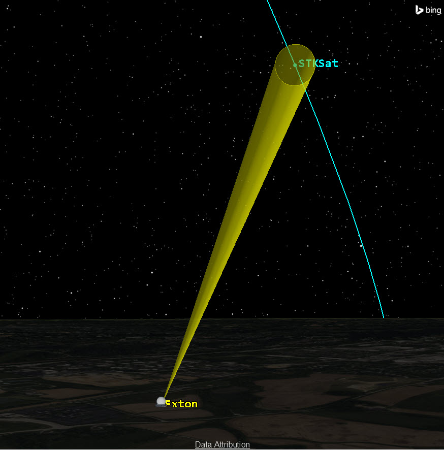
Exton's Sensor tracking STKSat
Modeling the ground site's VHF transmitter
Modeling transmitters involves configuring the output power of the system, the modulation technique being utilized, system losses, data rate, and properties of the antenna connected to the transmitter.
Inserting a Transmitter object
Attach a Transmitter (![]() ) object to AntennaRotor (
) object to AntennaRotor (![]() ). The ground site will be sending commands up to the satellite for this mission.
). The ground site will be sending commands up to the satellite for this mission.
- Insert a Transmitter (
 ) object using the Insert Default () method.
 - Select AntennaRotor () in the Select Object window.
- Click .
- Rename Transmitter1 () VHF_ExtonTx.
Configuring the VHF transmitter model
The ground site will transmit in the very high frequency (VHF) range with a custom power and data rate. Configure the transmitter to use a
- Open VHF_ExtonTx's () Properties ().
- Select the Basic – Definition page when the Properties Browser opens.
- Click the Transmitter Model Component Selector (
 ).
). - Select Complex Transmitter Model (
 ) from the Transmitter Models list when the Select Component dialog box opens.
 - Click to accept your changes and to close the Select Component dialog box.
- Select the Model Specs tab.
- Set the following options:
- Click to save your changes and to keep the Properties Browser open.
| Option | Value |
|---|---|
| Frequency | 145 MHz |
| Power | 20 dBW |
| Data Rate | 9600 b/sec |
Configuring the antenna polarization
Modify the polarization of the transmitter's antenna to Right-hand Circular to model a Yagi-Uda antenna. Yagi antennas are typically either right-hand or left-hand circularly polarized.
- Select the Antenna tab.
- Select the Polarization subtab.
- Select the Use check box.
- Change the polarization to Right-hand Circular.
- Click .
Setting the transmitter's modulation technique
Set the transmitter to use MSK modulation.
- Select the Modulator tab.
- Select MSK from the Name drop-down list as the modulating technique.
- Ensure the Auto Scale check box is selected in the Signal Bandwidth panel.
This option automatically calculates the bandwidth of the signal based on the frequency, data rate, and modulation technique.
- Click .
Modeling the ground site's UHF receiver
Modeling receivers involves configuring the internal and external system losses, the system noise temperature, the demodulation technique to be used, and properties of the antenna connected to the receiver.
Inserting a Receiver object
Attach a Receiver (![]() ) object to AntennaRotor (
) object to AntennaRotor (![]() ). The ground site will be receiving images from the satellite during this mission.
). The ground site will be receiving images from the satellite during this mission.
- Insert a Receiver (
 ) object using the Insert Default () method.
 - Select AntennaRotor () in the Select Object window.
- Click .
- Rename Receiver1 () UHF_ExtonRx.
Configuring the UHF receiver model
Use a
- Open UHF_ExtonRx's () Properties ().
- Select the Basic – Definition page.
- Click the Receiver Model Component Selector ().
- Select Complex Receiver Model () in the Select Component dialog box.
- Click .
- Select the Model Specs tab.
- Clear the Auto Track check box.
- Set the following options:
- Click .
| Option | Value |
|---|---|
| Frequency | 435 MHz |
| Antenna to LNA Line Loss | 3 dB |
| LNA Gain | 20 dB |
| LNA to Receiver Line Loss | 2 dB |
Configuring the receiver antenna's polarization
Modify the polarization of the receiver's antenna to model a Yagi-Uda antenna.
- Select the Antenna tab.
- Select the Polarization subtab.
- Select the Use check box.
- Change the polarization to Right-hand Circular.
- Click .
Setting the system noise temperature
The Receiver's System Noise Temperature allows you to specify the system's inherent noise characteristics. These settings can more accurately simulate real-world RF conditions.
- Select the System Noise Temperature tab.
- Select the Compute check box.
- Set the following options:
- Select the Constant check box in the Antenna Noise panel.
- Set the Antenna Noise - Constant to 1200 K.
- Click .
| Option | Value |
|---|---|
| Antenna to LNA Transmission Line - Temperature | 290 K |
| LNA - Noise Figure | 2 dB |
| LNA - Temperature | 60 K |
| LNA to Receiver Transmission Line - Temperature | 130 K |
For a higher-fidelity analysis, using the Compute option is preferred; for the sake of consistency in this exercise, you are using a constant value instead.
Configuring the demodulator and filter
The demodulator and the filter are the remaining settings that you will change.
- Select the Demodulator tab.
- Clear the Auto-select Demodulator check box.
- Select MSK in the Name drop-down list as the demodulating technique.
- Select the Filter tab.
- Ensure the Auto Scale check box is selected in the Receiver Bandwidth panel.
- Click .
Modeling the satellite's UHF transmitter
The STKSat satellite uses a CPUT VUTRX transceiver, comprised of a VHF uplink receiver and a UHF downlink transmitter. The transmitter specs are as follows:
| Characteristic | Value |
|---|---|
| Transmitter Output Power | Adjustable, 27–33 dBm |
| Transmit Power Draw | 4–10 W (27–33 dBm) |
| Data Rate | 9,600 baud (same as b/sec) |
| Modulation | GMSK/MSK |
Use these values to model the UHF transmitter portion of the transceiver with a Transmitter (![]() ) object.
) object.
Inserting a Transmitter object
Attach a Transmitter (![]() ) object to STKSat (
) object to STKSat (![]() ).
).
- Insert a Transmitter () object using the Insert Default () method.
- Select STKSat () in the Select Object dialog box.
- Click .
- Rename Transmitter2 () UHF_SatTx.
Configuring the UHF transmitter model
STKSat's transceiver transmits in the ultra high frequency (UHF) range, with a custom power, and data rate. Use a Complex Transmitter model to model configured for these specifications.
- Open UHF_SatTx's () Properties ().
- In the Properties window, select the Basic – Definition page.
- Change the Transmitter Model to a Complex Transmitter Model () in the Component Selector.
- Select the Model Specs tab.
- Set the following options:
- Click .
| Option | Value |
|---|---|
| Frequency | 435 MHz |
| Power | 3 dBW |
| Data Rate | 9600 b/sec |
Configuring the transmitter antenna's polarization
Modify the polarization of the transmitter's antenna to model an onboard Yagi-Uda monopole antenna. Change the polarization to Right-hand Circular.
- Select the Antenna tab.
- Select the Polarization subtab.
- Select the Use check box.
- Change the polarization to Right-hand Circular.
- Click .
Setting the transmitter's modulation
Set the transmitter to use the MSK modulation technique.
- Select the Modulator tab.
- Select MSK in the Name drop-down list.
- Ensure the Auto Scale check box is selected in the Signal Bandwidth panel.
- Click .
Modeling the satellite's VHF receiver
The STKSat satellite uses a CPUT VUTRX transceiver, comprised of a VHF uplink receiver and a UHF downlink transmitter. The receiver specs are as follows:
| Characteristic | Value |
|---|---|
| Receiver Sensitivity | -120 dBm |
| Receiver Power Draw | 250 mW |
| Data Rate | 9,600 baud |
| Modulation | GMSK/MSK |
Use these values to model the VHF uplink receiver portion of the transceiver with a Receiver object.
Inserting a Receiver object
Attach a Receiver object to STKSat. The Satellite will be receiving commands from the ground site during the mission.
- Insert a Receiver () object using the Insert Default () method.
- Select STKSat () in the Select Object dialog box.
- Click .
- Rename Receiver2 () VHF_SatRx.
Configuring the VHF receiver model
Use a Complex Receiver model for the satellite's receiver.
- Open VHF_SatRx's () Properties ().
- Select the Basic – Definition page.
- Change the Receiver Model to a Complex Receiver Model () in the Component Selector.
- Select the Model Specs tab.
- Clear the Auto Track check box.
- Set the Frequency to 145 MHz.
- Click .
Configuring the receiver antenna's polarization
Modify the polarization of the receiver to model an onboard Yagi-Uda monopole antenna. Change the polarization to Right-hand Circular.
- Select the Antenna tab.
- Select the Polarization subtab.
- Select the Use check box.
- Change the polarization to Right-hand Circular.
- Click .
Setting the system noise temperature
Specify the receiver's inherent noise characteristics to better simulate real-world RF situations.
- Select the System Noise Temperature tab.
- Select the Compute check box.
- Set the following options:
- Select the Constant option in the Antenna Noise panel.
- Set the Antenna Noise - Constant to 1200 K.
- Click .
| Option | Value |
|---|---|
| Antenna to LNA Transmission Line - Temperature | 290 K |
| LNA - Noise Figure | 1 dB |
| LNA - Temperature | 1000 K |
| LNA to Receiver Transmission Line - Temperature | 290 K |
Configuring the receiver's demodulator and filter
The demodulator and the filter settings.
- Select the Demodulator tab.
- Clear the Auto-select Demodulator check box.
- Select MSK in the Name drop-down list.
- Select the Filter tab.
- Ensure the Auto Scale check box is selected in the Receiver Bandwidth panel.
- Click .
Including additional gains and losses
Model the pre-receive and pre-demodulation losses in STKSat's receiver. The first loss is due to antenna coupling, polarization, etc., due to the satellite's inability to point the receiver. The pre-modulation loss represents losses inside the receiver system between the antenna and the demodulator. This loss is due to size and technology constraints.
- Select the Additional Gains and Losses tab.
- Click in the Pre-Receive Gains/Losses panel.
- Click in the Gain cell.
- Update the Gain value to -15 dB.
- Click in the Pre-Demodulation Gains/Losses panel.
- Change the Gain value to -8 dB.
- Click .
This represents a pre-receive loss due to antenna coupling, polarization, etc. This loss is greater due to the lack of pointing capability.
This represents losses inside the receiver system between the antenna and the demodulator. This loss is also greater for satellites due to size and technology constraints.
Simulating the ground site’s Yagi-Uda antennas with the Ansys HFSS Antenna Design Toolkit
Within the
Use the HFSS Antenna Design Toolkit to simulate two wire Yagi-Uda antennas in a vacuum for use with the Exton ground site, one designed for the VHF transmitter frequency of 145 MHz, and the other for the UHF receiver frequency of 435 MHz.
If you do not have access to the AEDT platform and the HFSS software, skip to the
Opening the HFSS Antenna Design Toolkit in the AEDT platform
Open the Antenna Toolkit in the AEDT platform.
- Open the Ansys Electronics Desktop (AEDT) application.
- Select the View tab.
- Select ACT Extensions in the Docking Windows drop-down menu on the View ribbon.
- Click Launch Wizards when the ACT Extensions window opens.
- Click HFSS Antenna Toolkit to open the Antenna Wizard.
Designing Exton's VHF antenna with the HFSS Antenna Wizard
Use the HFSS Antenna Wizard to synthesize Exton's wire Yagi-Uda VHF antenna.
- Launch the HFSS Antenna Toolkit in the ACT Extensions window.
- Expand Yagi-Uda in the library list on the left side of the Antenna Toolkit.
- Select Wire Yagi-Uda.
- Enter 0.145 for the Center Frequency. This will be your VHF antenna.
- Click .
- Click to generate the antenna. This will take a few seconds to load.
- Close the ACT Extensions window and maximize the project window.
You will see the dimensions of the antenna shrink to reflect the high operating frequency. Antenna size is directly related to its signal’s wavelength, making it inversely proportional to frequency.
Viewing the VHF antenna's excitations
In the HFSS software, excitations are sources of electromagnetic fields in a design. By assigning excitations, you define sources of electromagnetic fields, including antennas.
- Expand (
 ) Excitations in the Project Manager.
 - Select the 1 Excitation to display its properties in the Properties Window.
- Note that its impedance is 50 ohms by default.
Updating the VHF antenna's excitations
To get the results to align between the STK and HFSS software, you need to inject 1 W of incident power from the source impedance driving the antenna design in the HFSS application. You can do this by calculating the peak incident voltage ( Vpk ) for your incident power ( Pin ) that is equal to 1 W with an impedance ( Rsource ) of 50 ohms. Since

and the peak incident voltage you need is 10 V.
- Right-click on Excitations in the Project Manager.
- Select Edit Sources... in the shortcut menu.
- Click on the Magnitude Field on the Spectral Fields tab when the Edit post process sources dialog box opens.
- Enter 10 in the Magnitude Field.
- Ensure the Unit is set to V.
- Ensure the Incident Voltage option is selected for Terminal Excitation Type.
- Ensure the Use Maximum Available Power option is selected for System power for gain calculations.
- Click to accept your changes and to close the Edit post process sources dialog box.
You could also correct for these missing losses in the STK application by entering a value (in dB) in the User Gain Factor field to artificially offset the magnitude of the entire gain pattern. You can find this field by opening a transmitter or receiver object's properties, selecting the Basic - Definition page, selecting the Antenna tab, and then the Model Specs subtab.
Analyzing and validating the VHF antenna design
Before you export your antenna, first analyze the design and validate it to check for vaults that could jeopardize its accuracy.
- Select the Simulation tab.
- Click Validate.
- Click when the check is complete
- Click Analyze All on the Simulation ribbon to analyze your design. This may take a few minutes to compute.
Exporting the VHF antenna pattern
Now that your antenna design has been analyzed and validated, export your antenna pattern for further simulation with the STK software.
- Expand () Radiation in the Project Manager.
- Right-click on 3D.
- Select Compute Antenna Parameters... in the shortcut menu.
- Click .
- Name the file Exton_YagiUda_VHF.ffd.
- Click .
- Click to close the Antenna Parameters dialog box.
- Click Save in the ribbon to save your project.
Designing Exton's UHF antenna with the HFSS Antenna Wizard
Use the HFSS Antenna Wizard to synthesize Exton's wire Yagi-Uda UHF receiver antenna.
- Relaunch the HFSS Antenna Wizard from the ACT Extensions window.
- Expand Yagi-Uda in the library list on the left side of the Antenna Toolkit.
- Select Wire Yagi-Uda.
- Enter 0.435 for the Center Frequency. This will be your UHF antenna.
- Click .
- Click to generate the antenna.
- Close the ACT Extensions window and maximize the project window.
- Note that a new project, WireYagiUda_ATK2, has been created for the UHF antenna.
Updating the UHF antenna's excitations
To model the antenna pattern, you must also adjust the peak incident voltage for use with the STK application. As with the VHF antenna, you will use the default impedance is 50 ohms.
- Right-click on WireYagiUda_ATK2 - WireYagiUda_ATK (Hybrid Terminal Network) - Excitations in the Project Manager.
- Select Edit Sources... in the shortcut menu.
- Click in the Magnitude Field on the Spectral Fields tab when the Edit post process sources dialog box opens.
- Enter 10 in the Magnitude Field
- Ensure the Unit is set to V.
- Ensure the Incident Voltage option is selected for Terminal Excitation Type.
- Ensure Use Maximum Available Power option is selected for System power for gain calculations.
- Click to accept your changes and to close the Edit post process sources dialog box.
Analyzing and validating the UHF antenna design
Analyze the antenna design and validate it to check for vaults before exporting.
- Expand () Radiation in the Project Manager.
- Select the Simulation tab.
- Click Validate on the Simulation ribbon.
- Click when the check is complete to close the Validation Check dialog box.
- Click Analyze All on the Simulation ribbon to analyze your design.
Exporting the UHF antenna pattern
Now that your antenna design has been validated, export your antenna pattern as a FFD file.
- Expand () Radiation in the Project Manager.
- Right-click on 3D.
- Select Compute Antenna Parameters... in the shortcut menu.
- Click .
- Name the file Exton_YagiUda_UHF.when the Save As dialog box appears.
- Click to create the file and close the Save As dialog box.
- Click to close the Antenna Parameters dialog box.
- Click Save in the ribbon.
Simulating the satellite’s antennas with the Ansys HFSS SBR+ software
Antennas operating on large host platforms can experience significant performance degradation due to electromagnetic interaction with their host structure. The installation placement of the antenna will significantly affect the overall efficiency of the wireless communication or radar systems that these antennas service.
Instead of computing an antenna pattern in a vacuum in the same way as the Yagi-Uda antennas for the ground site, you can simulate and study installed antenna applications using the
STKSat's antennas must take into account the obstructions from the satellite platform. Use the SBR+ software to see how the STKSat satellite model itself interferes with the antenna gain in all directions.
Setting up a new HFSS design
Create a new project in the AEDT platform for modeling the STKSat's antennas.
- Open the Ansys Electronics Desktop (AEDT) application.
- Select the Desktop tab.
- Click New on the Desktop ribbon to create a new AEDT project.
- Right-click on the project.
- Select Rename.
- Name the project STKSat.
- Right-click on the project.
- Select Insert in the shortcut menu.
- Select Insert HFSS Design in the Insert submenu. The 3D Model window will appear.
Setting up the Modeler
Set up your AEDT project to use the HFSS SBR+ software for modeling.
- Select the Modeler command in the menu bar.
- Select Units....
- Select meter in the Select units drop-down menu when the Set Model Unites and Max Extent dialog box appears.
- Click to change the units to meters and to close the Set Model Unites and Max Extent dialog box.
- Select the HFSS command in the menu bar.
- Select Solution Type….
- Select SBR+ in the Solutions Types panel when the Solution Types: Project STKSat - HFSSDesign1 dialog box appears.
- Click to confirm your selection and to close the Solution Types: Project STKSat - HFSSDesign1 dialog box.
- Click Save to save your project.
Preparing the HFSS import options
Additional HFSS import options need to be enabled before you can import your satellite model.
- Select the Tools command in the menu bar.
- Select Options.
- Select General Options... in the Options submenu.
- Expand () General in the Options list.
- Select the Desktop Configuration page.
- Click .
- Scroll to the HFSS Feature Names when the Beta Options dialog box opens.
- Select the check boxes for HFSS Auto HPC NUMA support, HFS Cable Modeling, HFSS Nonlinear Drude for Implicit Transient, and HFSS PI.
- Click to confirm your selection and to close the Beta Options dialog box.
- Click to confirm your changes and to open the Ansys Electronics Desktop dialog box.
Restarting the Ansys Electronics Desktop platform
For the modified beta options to take effect, the AEDT platform needs to be restarted.
- Click to close the Ansys Electronics Desktop dialog box and to restart the platform.
- Select the Desktop tab.
- Click the downward-facing arrow below Open.
- Select STKSat.aedt in the drop-down menu to reopen your project.
Importing the satellite model
Import the satellite model into the modeler for SBR simulation.
- Select the Modeler command in the menu bar.
- Select Import….
- Navigate to your scenario folder.
- Select the STKSatModel.stl stereolithography file modeling the surface geometry of the STKSat satellite you downloaded at the start of this lesson.
- In the Facet Import Options panel, select the check boxes for Heal and Import as Lightweight Faceted Body. This will help speed things up, especially since this a shooting and bouncing ray simulation.
- Click to load the model and open the 3D Modeler window.
- The model will load into the Modeler View Area of the 3D Modeler window. The History Tree in the left of the 3D Modeler window lists the active model's structure and grid details.
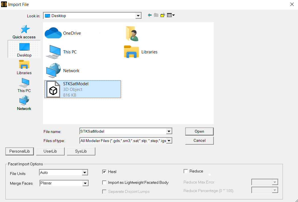
Facet import options in the Import File dialog box
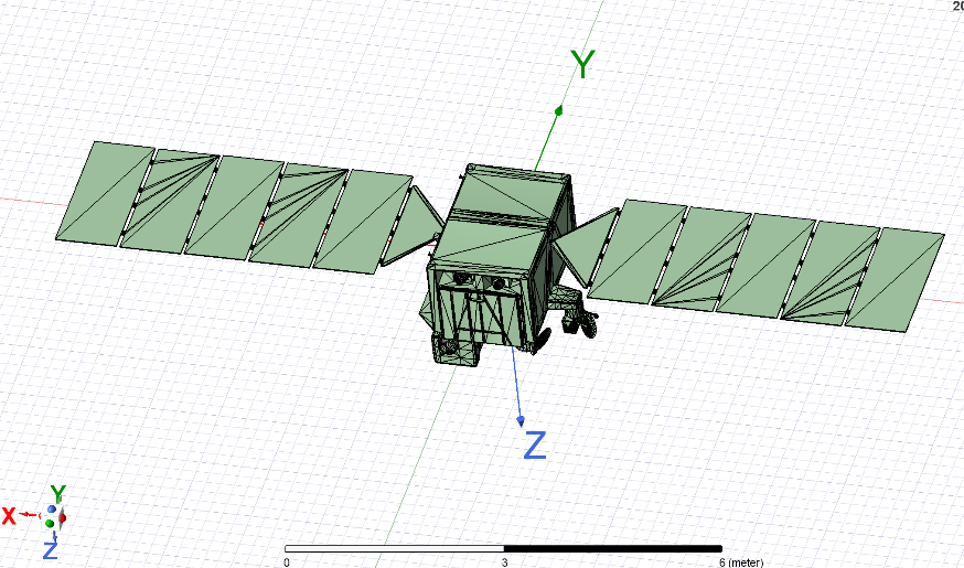
STKSatModel.stl in the model view Area
Assigning properties to the model
In order to validate the analysis, the model needs to have it’s material and boundary defined.
- Expand ()Model in the History Tree.
- Click on Sheets - Unassigned - STKSatModel. This will highlight the entire satellite model.
- Right-click Modeler View Area.
- Select Assign Boundary.
- Select Perfect E… in the Assign Boundary submenu.
- Click to confirm your selection and to close the Perfect E Boundary dialog box.
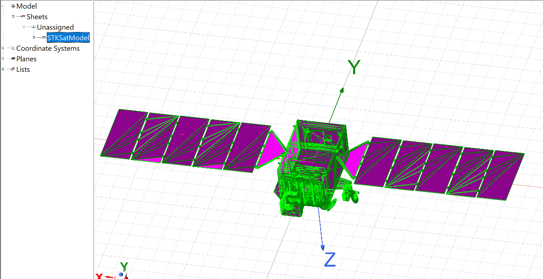
highlighted STKSAT model and history tree
Adding a relative coordinate system for the UHF antenna
Define a new relative coordinate system for the antenna. Antennas are attached at the origin of their assigned coordinate system.
- Zoom into the underside of the satellite. You should zoom in very close.
- Click Relative CS in the Draw Ribbon.
- A small square will appear under the cursor that highlights the snap point at any vertex you hover over. Click on a vertex near the bottom-left corner of the satellite model.
- The new relative coordinate system will appear with the Z axis pointing down. This needs to be fixed.
- Expand () Coordinate Systems in the History Tree.
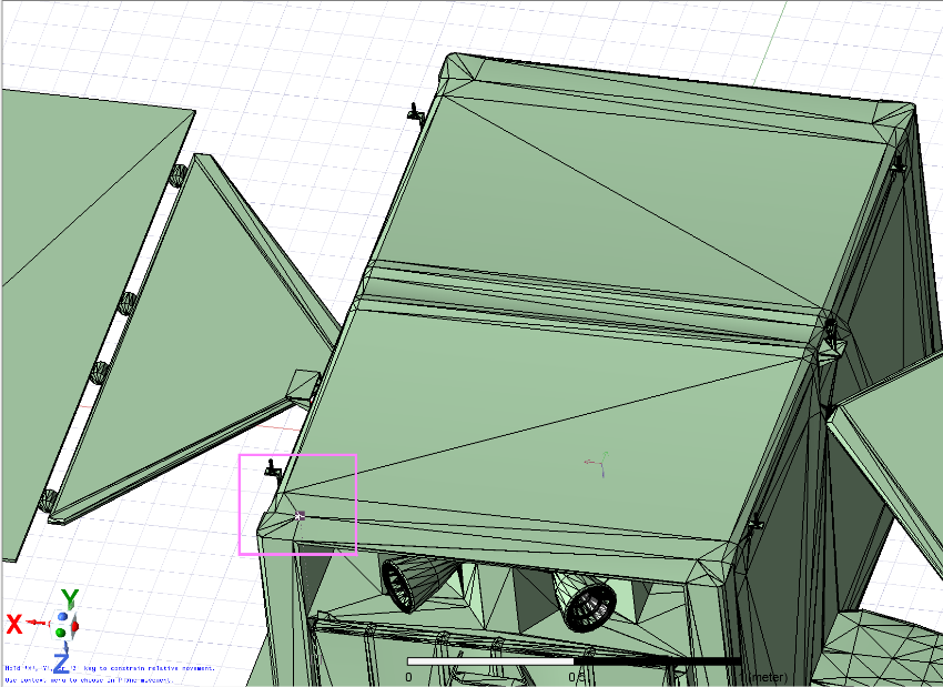
Underside of the STKSat Model showing the highlighted vertex for the new Relative CS
relative coordinate system for the STKSAT Model
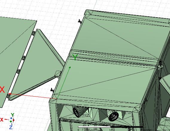
Updating the UHF coordinate system properties
It is important to ensure that you are modeling your antenna on the correct place on the satellite model and to ensure the axes are oriented correctly.
- Right-click on RelativeCS1.
- Select Properties... in the shortcut menu.
- Enter UHF_CS in the Name field when the Properties: Project STKSat - HFSSDesign1 - Modeler dialog box opens.
- In the Properties dialog box, change the X Axis property to 0 ,1 ,0.
- Change the Y Point property to 1 ,0 ,0.
- Set the Origin to 0.6237762581643 ,-1.0219597668976 ,-0.57153988427925.
- Click to accept your changes and to close the Properties dialog box. The Z axis will now be correctly orientated.

UHF relative CS Properties
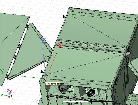
correctly oriented z axis
Updating the relative coordinate system for the VHF antenna
This first relative coordinate system was for the UHF antenna. Now, set up another reference coordinate system for the VHF antenna.
- Zoom in to the upper-right corner of the satellite.
- Select Global under Coordinate Systems in the History Tree. This is to allow the next reference coordinate system to reference the Global coordinate system, and not the one you just made.
- Click Relative CS in the Draw Ribbon.
- Click on the vertex on the top-right corner of the satellite to create your new relative coordinate system.
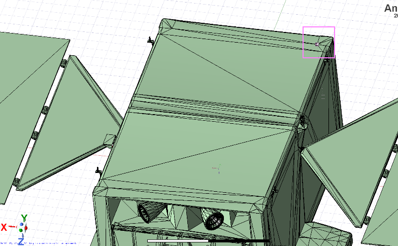
Node for the new VHF Relative CS
Updating the VHF coordinate system's properties
Update the relative coordinate system's properties to ensure the antenna is modeled at the correct place on the satellite with the correct orientation.
- Right-click RelativeCS1 in the History Tree.
- Select Properties... in the shortcut menu.
- Rename RelativeCS2 to VHF_CS.
- Change the X Axis property to 0 ,1 ,0 when the Properties: Project STKSat - HFSSDesign1 - Modeler dialog box opens.
- Change the Y Point property to 1 ,0 ,0.
- Set the Origin to -0.62374598620885 ,1.0217968642179 ,-0.57154787877286.
- Click to accept your changes and to close the Properties dialog box.
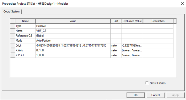
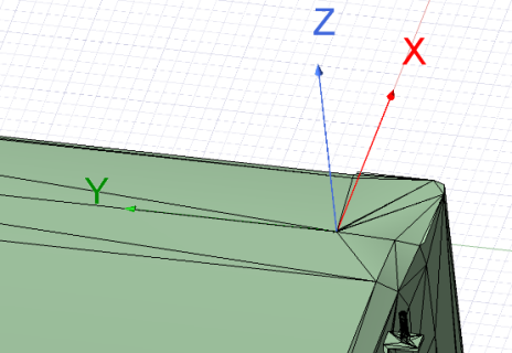
VHF_CS Properties and axes
Defining the UHF far-field setup
Define your far-field setup before generating the radiation patterns for your UHF antenna.
- Expand () HFSSDesign1 (SBR+).
- Right-click on Radiation in the Project Manager.
- Select Insert Far Field Setup in the shortcut menu.
- Select Infinite Sphere… in the Insert Far Field Setup submenu.
- Click on the Coordinate System tab once the Far Field Radiation Sphere Setup dialog box opens.
- Select Use local coordinate system.
- Select the UHF_CS in the Choose from existing coordinate systems... drop-down list.
- Click to confirm your selection and to close the Far Field Radiation Sphere Setup dialog box.
- Rename Infinite Sphere1 UHF.
Defining the VHF far-field setup
Repeat steps outlined in Defining the UHF far-field setup to create another infinite sphere referencing the VHF_CS coordinate system.
- Right-click on Radiation.
- Select Insert Far Field Setup in the shortcut menu.
- Select Infinite Sphere… in the Insert Far Field Setup submenu.
- Click on the Coordinate System tab.
- Select Use local coordinate system.
- Select the VHF_CS in the Choose from existing coordinate systems... drop-down list.
- Click .
- Rename Infinite Sphere2 VHF.
Defining the UHF excitations
For this exercise you will model a parametric wire monopole antenna using a current-source representation. Parametric antennas create far-field pattern sources that can provide S-parameter outputs and composite far-field radiation patterns; when using a current-source representation of the wire monopole, the axial current sources radiate in all directions, and the SBR software can correctly predict the interaction with the placement structure directly underneath because of the high-order fields imbedded in the current-source representation.
- Select UHF_CS in the History Tree.
- Right-click on Excitations in the project manager.
- Select Create Antenna Component in the shortcut menu.
- Select Wire Monopole… in the Create Antenna Component submenu.
- Enter UHF in the Name field once the Create Wire Monopole dialog box opens.
- Select Current Source.
- Change the Resonant Frequency to 0.435 GHz.
- Click .
- Click to accept your changes and to close the Create Wire Monopole dialog box.
Updating the UHF ground plane visualization
Though the HFSS software lets you model a signal layer as a ground plane, it is not needed for this analysis. Turn off its display in the 3D Modeler window.
- Expand () 3D Components in the Project Manager.
- Right-click on UHF1.
- Select Properties… in the shortcut menu.
- Select the Visualization tab when the Properties dialog box opens.
- Clear the Show Ground Plane - Value check box.
- Click to accept your changes and to close the Properties dialog box.
Defining the VHF excitations
Create an excitation called VHF with a resonant frequency of 0.145 GHz.
- Select VHF_CS in the History Tree.
- Right-click on Excitations in the project manager.
- Select Create Antenna Component in the shortcut menu.
- Select Wire Monopole… in the Create Antenna Component submenu.
- Enter VHF in the Name field.
- Select Current Source.
- Change the Resonant Frequency to 0.145 GHz.
- Click .
- Click .
Updating the VHF ground plane visualization
Turn off the display of the VHF ground plane in the 3D Modeler window.
- Expand () 3D Components in the Project Manager.
- Right-click on VHF1.
- Select Properties… in the shortcut menu.
- Select the Visualization tab when the Properties dialog box opens.
- Clear the Show Ground Plane - Value check box.
- Click to accept your changes and to close the Properties dialog box.
Adding the UHF solution setup
The last modeling step is to add the solution setup. Then, you can run the analysis.
- Right-click on Analysis in the Project Manager.
- Select Add Solution Setup… in the shortcut menu.
- Enter UHF in the Setup Name field when the SBR+ Solution Setup dialog box opens.
- Click in the Distribution field in the Frequency Sweeps panel.
- Select Single Point in the drop-down list.
- Change the frequency sweep to start at 0.435 GHz.
- Select the Compute Fields check box below the Frequency Sweeps panel.
- Select the Options tab.
- Select UHF from the drop-down list in the Field Observation Domain panel.
- Click to save your changes and to close the SBR+ Solution Setup dialog box.
Adding the VHF solution setup
Repeat these steps for a solution setup called VHF, with a frequency sweep of 0.145 GHz, and using the VHF field.
- Right-click on Analysis in the Project Manager.
- Select Add Solution Setup… in the shortcut menu.
- Enter VHF in the Setup Name field.
- Click in the Distribution field in the Frequency Sweeps panel.
- Select Single Point in the drop-down list.
- Change the frequency sweep to start at 0.145 GHz.
- Select the Compute Fields check box below the Frequency Sweeps panel.
- Select the Options tab.
- Select VHF from the drop-down list in the Field Observation Domain panel.
- Click .
Running the analysis
Now that you have set up solutions for both patterns, you can run your analysis.
- Select the Simulation tab.
- Click Analyze All on the Simulation ribbon.
Setting the post-process sources
Define the sources you will use to visualize the gain plots in the 3D Modeler window.
- Right-click on Excitations in the Project Manager.
- Select Edit Sources… in the shortcut menu.
- Select the Source Context tab when the Edit post process sources dialog box opens.
- Select the check boxes for both UHF1_p1 and VHF1_p1
- Click to accept your changes and to close the Edit post process sources dialog box.
Generating the UHF gain pattern
Build a 3D polar plot to visualize the UHF antenna pattern.
- Right-click on Results in the Project Manager.
- Select Create Far Fields Report in the shortcut menu.
- Select 3D Polar Plot in the Create Far Fields Report submenu.
- Select UHF1_P1 in the Sources menu in Context panel when the New Report - New Traces(s) dialog box opens.
- Ensure that the solution is set to the UHF : Sweep and that Geometry is referencing the UHF infinite sphere.
- Ensure the category is Gain, and the quantity is GainTotal.
- Select dB in the Function list.
- Click to generate the gain plot.
- Click to close the Report dialog box.
- Rename Gain Plot 1 UHF.
Generating the VHF gain pattern
Repeat these steps for a solution setup called VHF, with a frequency sweep of 0.145 GHz, and using the VHF field.
- Right-click on Results in the Project Manager.
- Select Create Far Fields Report in the shortcut menu.
- Select 3D Polar Plot in the Create Far Fields Report submenu.
- Select VHF : Sweep in the Solution menu.
- Ensure that Geometry is referencing the VHF infinite sphere.
- Select VHF1_P1 in the Sources menu.
- Select dB in the Function list.
- Click .
- Click .
- Rename Gain Plot 1 VHF.
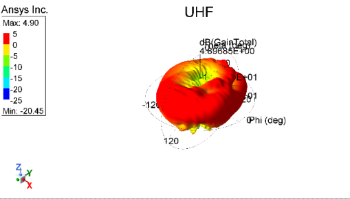
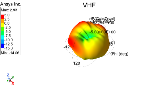
UHF and VHF Gain patterns
Visualizing the antenna gain patterns on the satellite
The antenna gain patterns can also be modeled on the satellite. This will help with orientation once brought into STK.
- Right-click on the UHF gain plot in the Project Manager.
- Select Show in Modeler Window in the shortcut menu.
- Repeat these steps for the VHF gain plot.
- Right-click on Field Overlays in the Project Manager.
- Select Plot Fields in the shortcut menu.
- Select Radiation Field....
- Reduce the scale for both plots to 0.1 when the Overlay Radiation Field dialog box opens.
- Click to save your changes.
- Click to close the Overlay Radiation Field dialog box
- Click HFSSDesign1 (SBR+) in the Project Manager to view the overlaid patterns.
The patterns are quite large and are overlapping, so they should be sized down. Note, this is purely for visuals, and is not changing anything about the actual results.
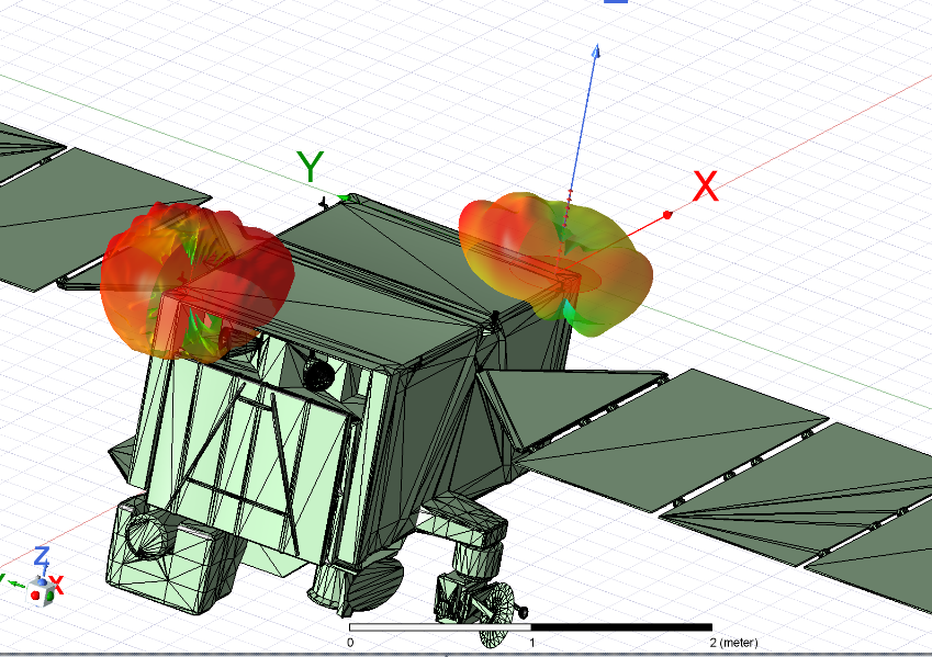
Antenna patterns modeled on the satellite
Defining the excitation source of the UHF antenna pattern
Before you can generate a pattern file for export, you must limit the source to just the UHF excitations.
- Right-click on Excitations in the Project Manager.
- Select Edit Sources… in the shortcut menu.
- Set the magnitude for the UHF excitation to 1 and the magnitude for the VHF excitation to 0.
- Ensure the Unit is set to W.
- Click .
To align the results between the STK and HFSS software, you need to inject 1 W of incident power from the source impedance driving the antenna design, as STK operates on a baseline assumption of 1 W of incident power.
Exporting the UHF gain pattern as a FFD file
Now that you have defined your sources, you can compute the antenna parameters and produce a FFD file modeling the UHF antenna gain pattern that can be imported into the STK application.
- Expand () Radiation in the Project Manager.
- Right-click on UHF.
- Select Compute Antenna Parameters... in the shortcut menu.
- Ensure that the Solution is set to UHF : Sweep and Intrinsic Variation is set to Freq=0.435GHz when the Antenna Parameters dialog box opens.
- Click
- Name the file STKSatModel_UHF.ffd.
- Click .
- Click to close the Antenna Parameters dialog box.
Defining the excitation source of the VHF antenna pattern
Limit the excitation source just to the VHF frequency.
- Right-click on Excitations in the Project Manager.
- Select Edit Sources… in the shortcut menu.
- Set the magnitude for the VHF excitation to 1 and the magnitude for the UHF excitation to 0.
- Ensure the Unit is set to W.
- Click .
Exporting the VHF gain pattern as a FFD file
Now that you have defined your sources, you can compute the antenna parameters and produce the FFD file modeling the VHF antenna gain pattern.
- Expand () Radiation in the Project Manager.
- Right-click on VHF.
- Select Compute Antenna Parameters... in the shortcut menu.
- Ensure that the Solution is set to VHF : Sweep and Intrinsic Variation is set to Freq=0.145GHz.
- Click
- Name the file STKSatModel_VHF.ffd
- Click .
- Click .
- Click Save in the ribbon.
- Close the AEDT platform.
Importing and configuring the antennas in the STK application
You can import
- Exton_YagiUda_UHF.ffd
- Exton_YagiUda_VHF.ffd
- STKSatModel_UHF.ffd
- STKSatModel_VHF.ffd
If you used the HFSS Antenna Wizard and the SBR+ software to generate your antenna patterns, use the FFD files you produced in the Simulating the ground site’s Yagi-Uda antennas with the Ansys HFSS Antenna Design Toolkit and Simulating the satellite’s antennas with the Ansys HFSS SBR+ software sections. If not, use the four FFD files included with the starter scenario.
Importing the ground site UHF receiver antenna pattern
Import the antenna pattern for Exton's UHF receiver.
- Open UHF_ExtonRx's () Properties ().
- Select the Basic - Definition page.
- Select the Antenna tab.
- Select the Model Specs subtab.
- Change the Antenna Model to ANSYS ffd Format () in the Component Selector.
- Click the ellipsis () next to External Filename.
- Browse to the location of your Far Field Data files.
- Select Exton_YagiUda_UHF.ffd when the Select File dialog box opens.
- Click to set the antenna model to use the external pattern file and to close the Select File dialog box.
- Click .
Orienting the ground site UHF receiver antenna pattern
The pattern needs to be rotated to align with the axes in the STK application. You want the antenna gain pattern to match the direction of the sensor.
- Select the Orientation subtab.
- Select YPR Angles from the Orientation drop-down list
- Enter the following parameters:
- Click .
| Parameter | Position Offset |
|---|---|
| Yaw | 90 deg |
| Pitch | 90 deg |
| Roll | 0 deg |
Visualizing the ground site UHF receiver antenna pattern
The hot part of the gain should point along the sensor pointing direction. In order the check this, the graphics for the volume have to be turned on.
- Select the 3D Graphics - Attributes page.
- Select Show Volume in the Volume Graphics panel.
- Set the Minimum Displayed Gain to -48 dB.
This value corresponds to the minimum gain displayed on the 3D System Gain Plot of the antenna pattern in the HFSS software.
- In the Pattern panel, set the Elevation - Stop angle to 180 deg.
- Click to save your changes.

UF3 3D Gain Plot in the HFSS software
Reviewing your changes
- Click Start () on the Animation Toolbar to animate your scenario.
- Pause (
 ) the animation when the satellite is overhead.
 - View the antenna pattern in the 3D Graphics window.
- If this orientation does not work, keep changing the angle in increments of 90 degrees until it aligns.

visualized Ground site Antenna pattern
Importing the ground site VHF transmitter antenna pattern
Import the antenna pattern for the Exton's VHF transmitter.
- Open VHF_ExtonTx's () Properties ().
- Select the Basic - Definition page.
- Select the Antenna tab.
- Select the Model Specs subtab.
- Change the Antenna Model to ANSYS ffd Format () in the Component Selector.
- Click the ellipsis () next to External Filename.
- Browse to the location of your Far Field Data files.
- Select Exton_YagiUda_VHF.ffd when the Select File dialog box opens.
- Click .
- Click .
Orienting the ground site VHF transmitter antenna pattern
The pattern needs to be rotated to align with the axes in the STK application.
- Select the Orientation subtab.
- Select YPR Angles from the Orientation drop-down list.
- Enter the following parameters:
- Click .
| Parameter | Position Offset |
|---|---|
| Yaw | 90 deg |
| Pitch | 90 deg |
| Roll | 0 deg |
Visualizing the ground site VHF transmitter antenna pattern
As with the UHF pattern, hot part of the gain should point along the sensor pointing direction. In order the check this the graphics for the volume have to be turned on.
- Select the 3D Graphics - Attributes page.
- Select Show Volume in the Volume Graphics panel.
- Set the Minimum Displayed Gain to -55 dB.
- In the Pattern panel, set the Elevation - Stop angle to 180 deg.
- Click to save your changes.
Importing the satellite UHF transmitter antenna pattern
Import the antenna pattern for STKSat's UHF transmitter.
- Open UHF_SatTx's () Properties ().
- Select the Basic - Definition page.
- Select the Antenna tab.
- Select the Model Specs subtab.
- Change the Antenna Model to ANSYS ffd Format () in the Component Selector.
- Click the ellipsis () next to External Filename.
- Browse to the location of your Far Field Data files.
- Select STKSatModel_UHF.ffd when the Select File dialog box opens.
- Click to set the antenna model to use the external pattern file and to close the Select File dialog box.
- Click .
Orienting the satellite UHF transmitter antenna pattern
The pattern's position on the satellite needs to be offset to the location where it was modeled.
- Select the Orientation subtab.
- Select YPR Angles from the Orientation drop-down list.
- Leave the YPR angles at zero and enter the following position offset parameters:
- Click .
| Parameter | Position Offset |
|---|---|
| X | 0.4 m |
| Y | -0.7 m |
| Z | 0.8 m |
Visualizing the UHF satellite transmitter antenna pattern
Visualize the antenna pattern on STKSat in the 3D Graphics window.
- Select the 3D Graphics - Attributes page.
- Select Show Volume in the Volume Graphics panel.
- Set Gain Scale (per dB) to 3e-05 km.
- Set the Minimum Displayed Gain to -20 dB.
- In the Pattern panel, set the Elevation - Stop angle to 180 deg.
- Click to save your changes.
This decreases the size of the pattern for visualization purposes.
Importing the satellite VHF receiver antenna pattern
Import the antenna pattern for STKSat's VHF receiver.
- Open VHF_SatRx's () Properties ().
- Select the Basic - Definition page.
- Select the Antenna tab.
- Select the Model Specs subtab.
- Change the Antenna Model to ANSYS ffd Format () in the Component Selector.
- Click the ellipsis () next to External Filename.
- Browse to the location of your Far Field Data files.
- Select STKSatModel_VHF.ffd when the Select File dialog box opens.
- Click to set the antenna model to use the external pattern file and to close the Select File dialog box.
- Click .
Orienting the satellite VHF receiver antenna pattern
The pattern's position on the satellite needs to be offset to the location where it was modeled.
- Select the Orientation subtab.
- Select YPR Angles from the Orientation drop-down list.
- Leave the YPR angles at 0 and enter the following position offset parameters:
- Click .
| Parameter | Position Offset |
|---|---|
| X | -0.4 m |
| Y | 0.7 m |
| Z | 0.8 m |
Visualizing the satellite VHF receiver antenna pattern
Visualize the antenna pattern on STKSat in the 3D Graphics window.
- Select the 3D Graphics - Attributes page.
- Select Show Volume in the Volume Graphics panel.
- Set the Gain Scale (per dB) to 4e-05 km.
- Set the Minimum Displayed Gain to -14 dB.
- In the Pattern panel, set the Elevation - Stop angle to 180 deg.
- Click to save your changes.
Reviewing your changes
View the antenna patterns on STKSat in the 3D Graphics window.
- Right-click on STKSat () in the Object Browser.
- Select Zoom To in the shortcut menu.
- Move around the satellite to view the antenna patterns in place on the satellite model.
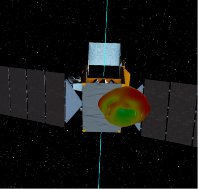
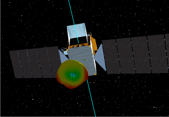
Visualized UHF and VHF gain patters on STKSat
Computing access between the transmitters and receivers
Access must be computed between two endpoints of an RF link in order to analyze the communications system. Compute access for both the VHF uplink and UHF downlink components.
Computing access for the VHF uplink
Compute access between the VHF transmitter on the ground site and the VHF receiver on the spacecraft.
- Right-click on VHF_ExtonTx () in the object browser.
- Select Access... (
 ) in the shortcut menu.
 - Expand () STKSat () in the Associated Objects list once the Access Tool opens.
- Select VHF_SatRx ().
- Click
 .
.
Computing access for the UHF downlink
Compute access between the UHF transmitter on the spacecraft and the UHF receiver on the ground site.
- Click to select a new object for which to compute access and to open the Select Object dialog box.
- Select UHF_SatTx () in the Select object list.
- Click to confirm your selection and to close the Select Object dialog box.
- Expand () Exton () in the Associated Objects list once the Access Tool opens.
- Expand () AntennaRotor ().
- Select UHF_ExtonRx ().
- Click .
- Close the Access Tool.
Generating detailed link budgets
Now that access has been computed between the UHF and VHF components of the communications system, you can generate and analyze your link budget for each link.
Generating a detailed link budget for the VHF uplink
Start by generating a detailed link budget report for the VHF uplink.
- Open the Analysis menu.
- Select Report & Graph Manager... (
 ).
). - Select Access in the Object Type drop-down list.
- Select the Facility-Exton-Sensor-AntennaRotor-Transmitter-VHF_ExtonTx-To-Satellite-STKSat-Receiver-VHF_ SatRx Access (
 ) object.
 - Select the Link Budget - Detailed report (
 ) in the Installed Styles (
 ) folder.
 - Click .
Reviewing the detailed link budget report
Review the results of the VHF link in the Link Budget - Detailed report.
- Scroll to the right of the report. Note the values of C/N, Eb/No, BER, and so on. Notice that the bit error rate (BER) values are very low numbers.
- Scroll back through the report and find the columns titles Freq. Doppler Shift (kHz) and Rcvd. Frequency (GHz).
- Change the units of the Rcvd. Frequency (GHz) column to MHz.
- Right click on the Rcvd. Frequency (GHz) title.
- Select Rcvd. Frequency in the shortcut menu.
- Select Units... (
 ) in the Received Frequency submenu.
 - Clear the Use Defaults check box when the Units dialog box opens.
- Select Megahertz (MHz) in the New Unit Value list.
- Click to apply your changes and to close the Units dialog box.
- Scroll down through the report and notice how the Rcvd. Frequency value shifts over time. This shift is called Doppler Shift. The Doppler Shift is the difference between the design frequency and the received frequency.
- Finally, scroll through the report and find the EIRP (dBW) and Prop Loss (dB) columns. Recall that the EIRP is the effective isotopic radiated power and that Prop Loss is signal loss as it travels from the transmitter to the receiver. In this case, the Prop Loss should be equal to the Free Space Loss as other environmental losses have not been modeled yet. The received isotropic power (RIP) is the difference between the EIRP and the propagation loss. The RIP is the received power at the receiver’s antenna.
- Keep the report open.
There are some very small bit error rates in the report. These outliers are somewhat unrealistic but indicate that the RF link between the ground site transmitter and the receiver on the spacecraft is strong at that point in time. These extremely small values indicate that there may be some loss not being accounted for. However, this is an acceptable report on this RF link since it gives us a comprehensive overview of the link as a whole.
In the STK software the RIP includes both the effect of propagation loss and the effect of bandwidth overlap. This overlap is caused by a mismatch between the transmitted signal’s bandwidth and the receiver bandwidth. This is another column shown in the link budget report style. This overlap may cause additional loss in calculations and thus a slightly weaker RIP.
Generating a detailed link budget for the UHF downlink
Generate a detailed link budget report for the UHF downlink.
- Return to the Report & Graph Manager ().
- Select the Satellite-STKSat-Transmitter-UHF_SatTx-To-Facility-Exton-SensorAntennaRotor-Receiver-UHF_ExtonRx Access () object.
- Select Link Budget - Detailed ().
- Click .
Reviewing the detailed link budget report
Review the results of the UHF link in the Link Budget - Detailed report.
- Scroll through the report and note the values of C/N, Eb/No, BER, and so on. Notice that the bit error rate (BER) values are larger. This is because the transmitter puts out much less power than a ground site transmitter.
- Scroll through the report and compare the link values from the UHF link to the VHF link analyzed previously. Note changes in Freq. Doppler Shift, Rcvd. Iso. Power, C/N, Eb/No, BER, and so on.
- Change the units of the Rcvd. Frequency (GHz) column to MHz.
- Right click on the Rcvd. Frequency (GHz) title
- Select Rcvd. Frequency in the shortcut menu
- Select Units... () in the Received Frequency submenu.
- Clear the Use Defaults check box.
- Select Megahertz (MHz) in the New Unit Value list.
- Click .
- Keep the report open.
Modeling environmental losses
An important aspect to modeling any RF link is modeling its losses. There are several built-in environmental models that allow modeling of losses due to rain, clouds and fog, atmospheric absorption, urban propagation, and so on. For satellites, rain, cloud, and atmospheric absorption models are the most applicable. Some of the models used are based on recommendations from the International Telecommunication Union (ITU). These recommendations overview the valid ranges and base equations of these models.
Enabling the environmental models
Enable the ITU RF environment models in your scenario.
- Open CommDesignStarter's () Properties ().
- Select the RF - Environment page.
- Select the Environmental Data tab.
- Select the Use ITU-R P.618 Section 2.5 check box in the Total Propagation Calculation tab.
This option allows the use of some other ITU models and calculates the total propagation loss in accordance with the ITU recommendation.
- Select the Rain, & Cloud & Fog tab.
- Select the Use check box in the Rain Model section. Ensure that the ITU-R P618-13 model is selected.
- Select the Use check box in the Clouds and Fog Model section. Ensure the ITU-R P840-7 model is selected.
- Select the Atmospheric Absorption tab.
- Select the Use check box.
- Click .
Ensure the ITU-R P676-9 model is selected.
Verifying rain model settings in the receiver objects
Ensure that the Use Rain Model check box is marked in both the receiver objects.
- Right-click on UHF_ExtonRx () in the Object Browser.
- Select Properties () in the shortcut menu.
- Select the Model Specs tab on the Basic - Definition page.
- Ensure that the Use check box is selected in the Rain Model panel.
- Click .
- Open VHF_SatRx's () Properties ().
- Select the Model Specs tab on the Basic - Definition page.
- Ensure that the Use check box is selected in the Rain Model panel
- Click .
Reviewing the changes in the link budget reports
You incorporated some environmental effects in your scenario. See the impact of these changes in your RF link in the detailed link budget reports.
- Return to the VHF Link Budget - detailed report window.
- Click the Refresh (
 ) at the top of the window to refresh the report data.
 - Return to the UHF Link Budget - detailed report window.
- Click the Refresh () at the top of the window to refresh the report data.
Notice the changes in C/N, Eb/No, and BER, the values should decrease because the environmental conditions have impacted the RF link. Scroll through the report and find the Atmos Loss (dB), Rain Loss (dB), and CloudsFog Loss (dB). Notice how these columns are now populated with dynamic data that changes over time.
Notice the changes in C/N, Eb/No, and BER, the values should decrease because the environmental conditions have impacted the RF link. Scroll through the report and find the Atmos Loss (dB), Rain Loss (dB), and CloudsFog Loss (dB). Notice how these columns are now populated with dynamic data that changes over time.
Calculating link margins and generating custom reports
Link margins are used to describe the strength of a signal. Typically, a threshold value for some link parameter such as EIRP, Eb/No, received power, etc. is set. Then, value of that link parameter at a point in time is compared to the threshold. The difference between the actual link value and the threshold is the link margin. Usually, the link margin threshold is set to a minimum value where the link closes. For example, receiver sensitivity defines the minimum signal strength a receiver can handle to maintain an RF link. When creating a link margin, the receiver sensitivity would be the link margin threshold. Then, the link margin value would tell you how close you are to that minimum strength. In the STK software, this can be done with communication constraints and custom link reports.
Setting the link margin threshold for VHF_SatRx
Change the settings for the VHF_SatRx.
- Open VHF_SatRx's () Properties ().
- Select the Model Specs tab on the Basic - Definition page.
- Select the Enable check box in Link Margin panel.
- Select Rcvd Carrier Power in the Type drop-down list.
- Set the Threshold field to -150 dBW
- Click .
Setting the link margin threshold for UHF_ExtonRx
Set the link margin for both receivers. First, change the settings for the UHF_ExtonRx.
- Open UHF_ExtonRx's () Properties ().
- Select the Model Specs tab on the Basic - Definition page.
- Select the Enable check box in Link Margin panel.
- Select Rcvd Carrier Power in the Type drop-down list.
- Set the Threshold field to -156 dBW.
- Click .
This is the sensitivity of the receiver on the ground site.
Examining the VHF uplink
Examine the Carrier to Noise Ratio (CNR) and Bit Error Rate (BER) for the two RF links. Since the RF links are represented as access calculations, examine those from the Report & Graph manager.
- Return to the Report & Graph Manager ().
- Ensure that Object Type is set to Access.
- Select the VHF Access () object.
- Generate the following graphs (
 ):
): - Carrier_to_Noise_Ratio
- Bit_Error_Rate
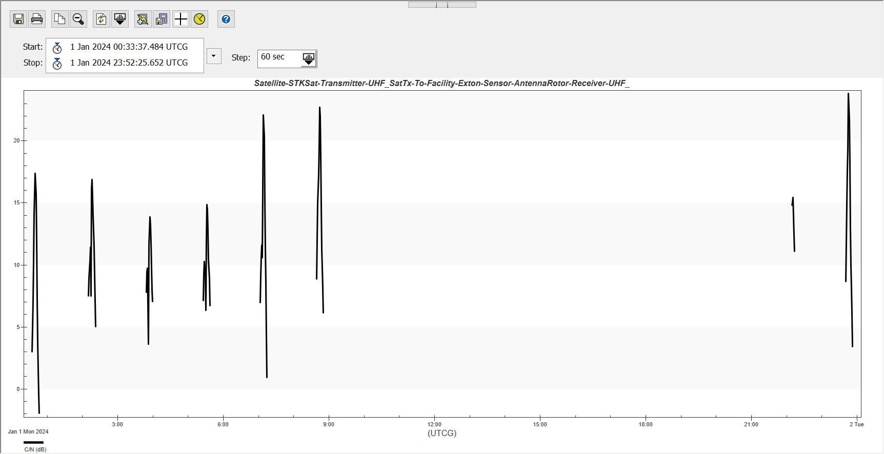
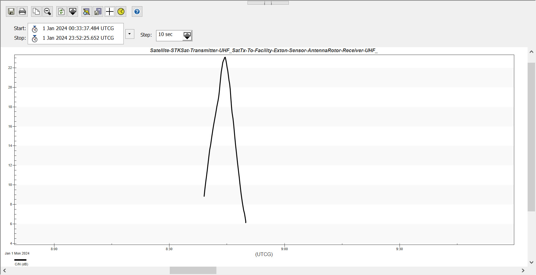
- In the Carrier to Noise Ratio graph, click and hold to draw a selection rectangle to around one of the peaks to zoom into one of the spikes.
- Decrease the time Step to 10 sec.
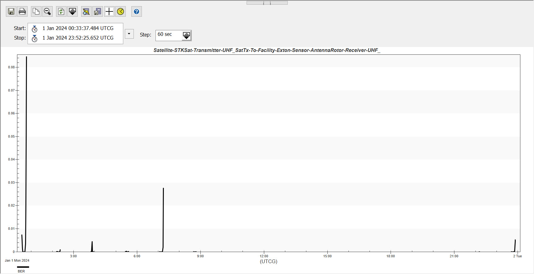
- The BER graph has spikes that represent areas of high bit error rates.
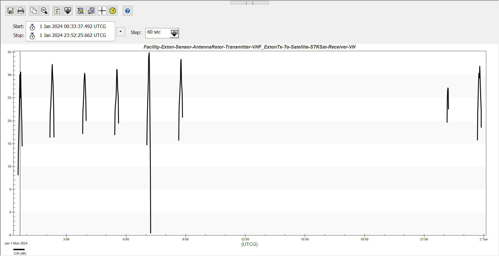
VHF Carrier to Noise Ratio Report
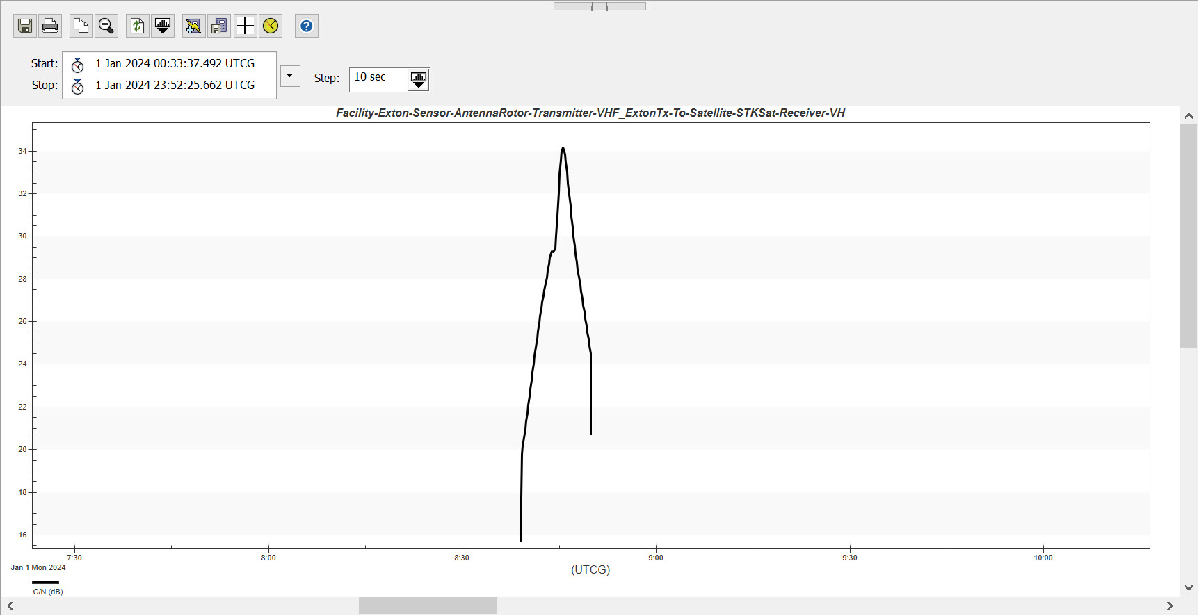
VHF Carrier to Noise Ratio Report zoomed in to a peak
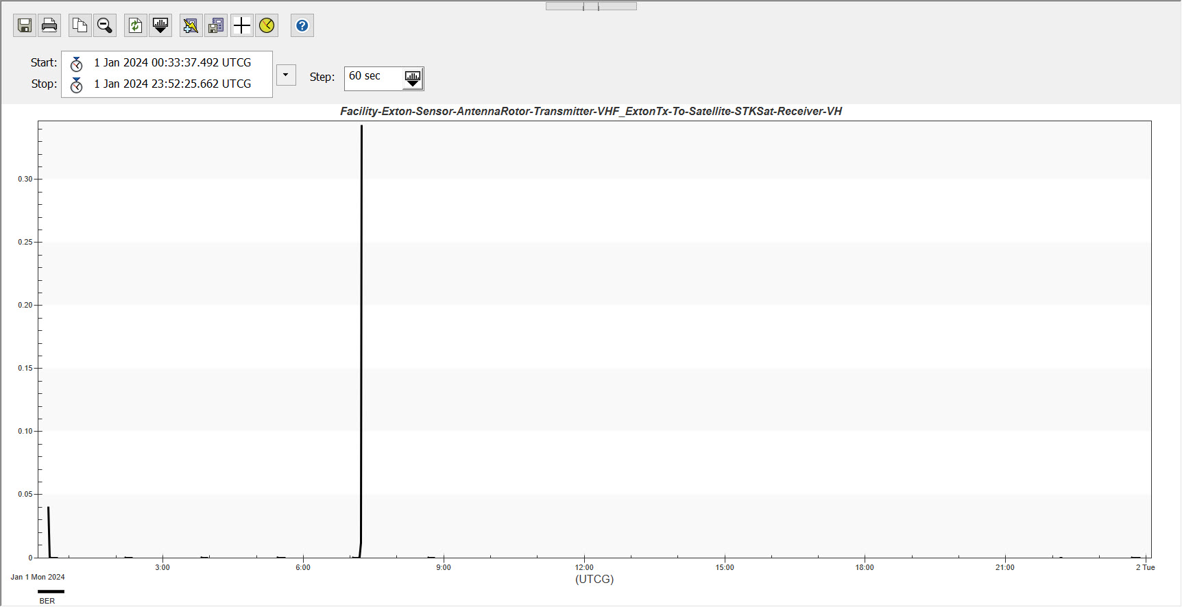
VHF BER Report
These brief moments represent when a link is just starting or ending. In other words, the connection is very bad when the satellite first comes into or is leaving the view of the sensor.
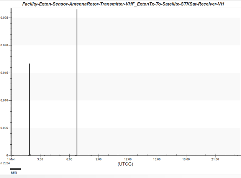
VHF BER Report showing twin SPIKES in the BER
Investigating the results
You can see from your data that the BER graph has spikes that represent areas of high bit error rates. These brief moments represent when a link is just starting or ending. In other words, the connection is very bad when the satellite first comes into or is leaving the view of the sensor.
- Right-click on the top of one of the spikes.
- Select Set Animation Time in the shortcut menu.
- Right-click on STKSat () in the Object Browser
- Select Zoom To in the shortcut menu.
- Bring the 3D Graphics window to the front.
- Zoom out from the satellite until you see the full sensor field of view.
- Move back and forth through time in the scenario. Watch as the satellite either comes just into the sensor's field of view or leaves it entirely.
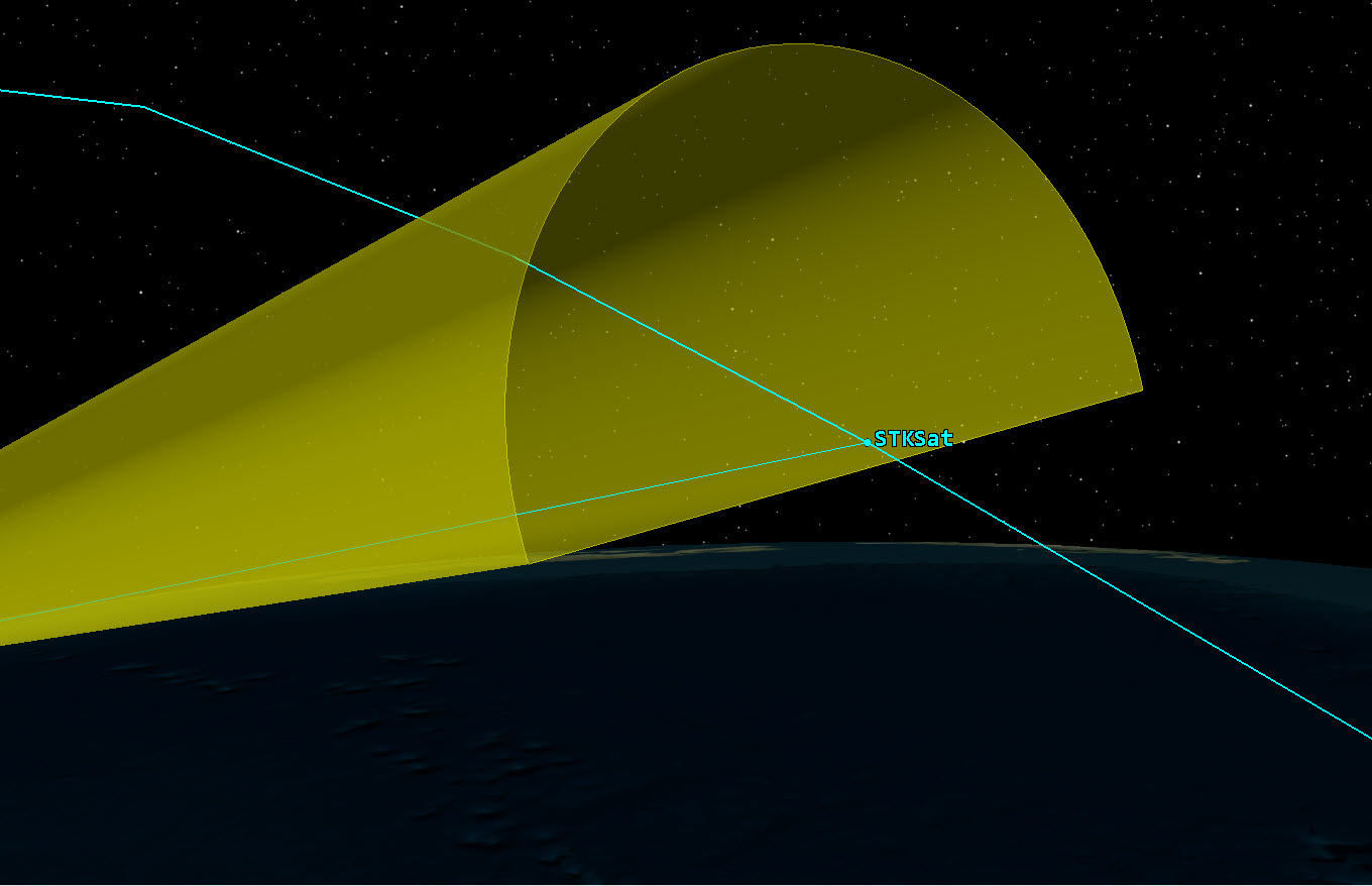
STKSat leaving the sensor's field of view
Examining the UHF downlink and investigating the results
Repeat these steps to generate and analyze the CNR and BER graphs for the UHF access object.
UHF Carrier to Noise Ratio report
UHF Carrier to Noise Ratio report zoomed in on a peak
UHF BER report
Creating custom link budget reports
Create a custom report using data providers that are important to your analysis.
Creating a new report style
Add a new report style for your custom link budget.
- Return to the Report & Graph Manager ().
- Ensure that Object Type is set to Access.
- Select Scenario Styles in the Styles list.
- Click Create new report style (
 ) in the Styles toolbar.
 - Name the report Custom Link Budget.
- Select the Enter key to open the report's properties.
Adding link Information data provider and elements
The Custom Link Budget report will include the Time, EIRP, Propagation Loss, Received Isotropic Power, Carrier Power at Receiver Input, Receiver Gain, Bit Error Rate, and Link Margin.
- Expand () the Link Information data provider ().
- Select the following data provider elements (
 ) in the Data Providers list to Insert () them into the Report Contents list in the order shown:
 - Time
- EIRP
- Prop Loss
- Rcvd. Iso. Power
- Carrier Power at Rcvr Input
- Rcvr Gain
- BER
- Link Margin
Setting options for data providers
Set the option for the data providers. The BER notations defaults to a Floating Point, change this to use Scientific notation.
- Select Link Information-BER in the Report Contents list.
- Click .
- Select Scientific (e) in the Notion drop-down menu in the Data Format panel when the Options: Section 1, Line 1, Link Information-BER dialog box opens.
- Click to accept your change and to close the Options: Section 1, Line 1, Link Information-BER dialog box.
- Click to accept your changes and to close the Report Style dialog box.
Generating the custom link budget reports
Examine the results for both RF links.
- Select the UHF Access () object.
- Select Custom Link Budget (
 ) in the Scenario Styles folder located in the Styles panel.
 - Click .
- Notice the format of the custom report and the new columns Carrier Power at Rcvr Input (dBW) and Link Margin (dB).
- Return to the Report & Graph Manager () window.
- Select the VHF Access () object.
- Select the Custom Link Budget () report style.
- Click .
Notice the Carrier Power at Rcvr Input and Link Margin values for this RF uplink.
Adding communications constraints
Constraints can be used to limit access calculations. For example, by default, there is a line-of-sight (LOS) constraint on all objects. Therefore, access is only determined to be possible when there is line of sight between objects. Additional communications constraints can be used to limit access to times when "acceptable” RF conditions exist. Common practice is requiring a link margin of at least 3 dB and a BER of at least 1e-03 to be maintained for the link to +be considered valid. These values can be used to constrain the data set to only show accesses that satisfy these requirements.
Constraining the UHF downlink
Add constraints to UHF_ExtonRx downlink receiver.
Adding constraints in versions 12.9 and later of the STK software
Add constraints to UHF_ExtonRx on the Constraints - Active page when using versions 12.9 and later of the STK software.
- Open UHF_ExtonRx's () Properties ().
- Select the Constraints - Active page.
- Click Add New Constraints (
 ).
). - Add the following constraints:
- Bit Error Rate
- Link Margin
- Power at Receiver Input
- Click .
- Select Bit Error Rate.
- Select the Max check box.
- Set the value to 1e-03.
- Clear the Min check box. Note that the Max constraint is used because a smaller BER is better.
- Select Link Margin.
- Select the Min check box.
- Set the value to 3 dB.
- Ensure the Max check box is cleared.
- Select Power at Receiver Input.
- Select the Min check box.
- Set the value to -156 dBW. This sets the minimum received power equal to the ground site receiver sensitivity.
- Ensure the Max check box is cleared.
- Click .
Adding constraints in versions 12.8 and earlier of the STK software
Add constraints to UHF_ExtonRx on the Constraints - Comm page when using versions of the STK software that are older than version 12.9.
- Open UHF_ExtonRx's () Properties ().
- Select the Constraints - Comm page
- Select the check boxes for the following constraints:
- Bit Error Rate
- Link Margin
- Power at Receiver Input
The Max constraint is used because a smaller BER is better. The Power at Receiver Input - Min value sets the minimum received power equal to the ground site receiver sensitivity.
- Enter the following values for the constraints:
- Click .
| Constraint | Value |
|---|---|
| Bit Error Rate - Max | 1e-03 |
| Link Margin - Min | 3 dB |
| Power at Receiver Input - Min | -156 dBW |
Viewing the constrained UHF downlink data
Review the custom link budget report for the UHF downlink to see the affects of the new constraints. If the report was previously opened, then simply refresh it to see the changes.
- Re-open the UHF downlink Custom Link Budget report.
- Click the Refresh () button to refresh the data.
Notice that the number of accesses and data points has decreased. Also, notice that all of the BER values are less than 1e-03 and the Link Margin values are all greater than 3 dB.
Constraining the VHF uplink
Repeat the process above to apply constraints to the VHF receiver on the satellite, the only change being a Minimum value for the Power at Receiver Input constraint of -150 dBW.
Adding constraints in versions 12.9 and later of the STK software
Add constraints to VHF_SatRx on the Constraints - Active page when using versions 12.9 and later of the STK software.
- Open VHF_SatRx's () Properties ().
- Select the Constraints - Active page.
- Click Add New Constraints ().
- Add the following constraints:
- Bit Error Rate
- Link Margin
- Power at Receiver Input
- Click .
- Select Bit Error Rate.
- Select the Max check box.
- Set the value to 1e-03.
- Clear the Min check box.
- Select Link Margin.
- Select the Min check box.
- Set the value to 3 dB.
- Ensure the Max check box is cleared.
- Select Power at Receiver Input.
- Select the Min check box.
- Set the value to -150 dBW.
- Ensure the Max check box is cleared.
- Click .
Adding constraints in versions 12.8 and earlier of the STK software
Add constraints to VHF_SatRx on the Constraints - Comm page when using versions of the STK software that are older than version 12.9.
- Open VHF_SatRx's () Properties ().
- Select the Constraints - Comm page.
- Select the check boxes for the following constraints:
- Bit Error Rate: Max
- Link Margin: Min
- Power at Receiver Input
- Enter the following values for the constraints:
- Click .
| Constraint | Value |
|---|---|
| Bit Error Rate - Max | 1e-03 |
| Link Margin - Min | 3 dB |
| Power at Receiver Input - Min | -150 dBW |
Viewing the constrained VHF uplink data
Review the custom link budget report for the VHF uplink to see the affects of the new constraints. If the report was previously opened, then simply refresh it to see the changes.
- Re-open the VHF uplink Custom Link Budget report.
- Click the Refresh () button to refresh the data.
Notice that the number of accesses and data points has decreased. Also, notice that all of the BER values are less than 1e-03 and the Link Margin values are all greater than 3 dB.
Optimizing the communications links
With the RF uplink and downlink established between the ground site and STKSat spacecraft, the various link parameters can be modified to optimize the link. These parameters include modulation technique, data rate, receiver sensitivity, and transmitter output power.
Modifying the modulation technique
In order to modify the modulation technique, the modulation settings for both the transmitter and receiver in a link must be modified.
- Open VHF_ExtonTx's () Properties ().
- Select the Basic – Definition page.
- Select the Modulator tab.
- Change the modulator Name field from MSK to FSK.
- Click .
- Return to the VHF uplink Custom Link Budget report.
- Refresh () the report.
Notice that when the modulator and demodulator do not match, the report shows that it has no data available. This is because the VHF receiver on the spacecraft is still configured for MSK modulation.
Modifying the demodulation technique
Change the demodulator on the receiver to FSK and refresh your report.
- Open VHF_SatRx's () Properties ().
- Select the Basic – Definition page.
- Select the Demodulator tab.
- Change the Name field from MSK to FSK.
- Click .
- Return to the VHF uplink Custom Link Budget report and refresh the data using the Refresh () button.
Notice the changes to the Bit Error Rate column. You now have better values for the BER. The Link Margin appears to be more evenly distributed across the data. This is due to the fact that the power spectral density (PSD) of FSK modulation is wider than that of MSK modulation
Modifying the UHF downlink
Repeat steps in Modifying the modulation technique and Modify the demodulator technique for the RF downlink (that is, modify the UHF_SatTx (![]() ) and UHF_ExtonRx (
) and UHF_ExtonRx (![]() ) objects). Notice that when the modulator and demodulator do not match the report has no data available. Once both the modulator and demodulator are set to FSK, refresh and examine the report.
) objects). Notice that when the modulator and demodulator do not match the report has no data available. Once both the modulator and demodulator are set to FSK, refresh and examine the report.
Modifying the transmitter data rate
Unlike the process of changing the modulation technique, the data rate options only need to be changed on transmitters in the RF link.
- Open UHF_SatTx's () Properties ().
- Select the Basic – Definition page.
- Select the Model Specs tab.
- Change the Date Rate from 9600 b/sec to 1200 b/sec.
- Click .
- Return to the UHF Custom Link Budget report.
- Refresh () the report.
Notice the changes in BER and Link Margin. A lower data rate corresponds to a lower (better) bit error rate. However, the Link Margin values have also decreased. This illustrates the tradeoff between signal bandwidth and power.
Modifying the VHF transmitter data rate
Repeat the steps in the Modifying the data rate section for the RF uplink (i.e. modify the VHF_ExtonTx (![]() ) object) and examine the report.
) object) and examine the report.
Modifying receiver sensitivity
The receiver sensitivity only needs to be changed for the receiver in an RF link. Because the ground site configuration is already established, only the receiver sensitivity on the STKSat spacecraft will be modified.
- Open VHF_SatRx's () Properties ().
- Select the Basic – Definition page.
- Select the Model Specs tab.
- Change the Link Margin - Threshold value from -150 dBW to -135 dBW.
- Click .
- Return to the VHF uplink Custom Link Budget report and refresh the data using the Refresh () button.
Notice the decreased access times and smaller Link Margin values due to the less-negative sensitivity value. The more-negative the sensitivity, the stronger the link.
Modifying transmitter output power
Similar to changing the data rate, the output power only needs to be changed for the transmitter in an RF link. Because ground sites typically just transmit at their maximum output power, only the output power for the transmitter on STKSat will be modified.
- Open UHF_SatTx's () Properties ().
- Select the Basic – Definition page.
- Select the Model Specs tab.
- Change the Power value from 3 dBW to 1 dBW.
- Click .
- Return to the UHF Custom Link Budget report and refresh the data using the Refresh () button.
Notice the link access times decrease due to the decreased transmit power. Also notice that the Link margin values decrease to very near the threshold value of 3 dB.
Saving your work
Clean up your workspace and save your scenario.
- Close all reports and windows except the 2D and 3D Graphics windows.
- Save (
 ) your work.
 - Close the scenario when done.
Summary
You created a custom antenna for the VHF and UHF frequency ranges, imported the antenna patterns designs created in the Ansys HFSS software into the STK application, and modeled their behavior in a multidomain mission. Using the HFSS SBR+ asymptotic high-frequency electromagnetic simulator and the STK software, you modeled the influence of physical obstacles near your antennas on the satellite and saw them reflected in a report. You analyzed a VHF uplink and a UHF downlink with these antennas using custom link budget reports. You then analyzed the link margins of the receiver sensitivity by optimizing the communications devices. When used together, you can create and analyze high-fidelity antenna models with the Ansys HFSS software and the STK application.