STK Premium (Space) or STK Enterprise
You can obtain the necessary licenses for this tutorial by contacting AGI Support at support@agi.com or 1-800-924-7244.
ModelCenter installation prerequisites: The ModelCenter software requires the installation of a 64-bit version of Java, a 64-bit implementation of Python 3.x, and the installation of the thrift and six Python packages. See the ModelCenter Installation Prerequisites for more information.
Required product install: The Ansys ModelCenter® model-based systems engineering software and the STK Plugin for ModelCenter are required to complete this tutorial.
This lesson requires version 13.0 of the STK software or newer to complete in its entirety. If you have an earlier version of the STK software, you can view a legacy version of this lesson.
This tutorial was written using version 2026 R1 of the Ansys ModelCenter® model-based systems engineering software.
The results of the tutorial may vary depending on the user settings and data enabled (online operations, terrain server, dynamic Earth data, etc.). It is acceptable to have different results.
Capabilities covered
This lesson covers the following capabilities of the Ansys Systems Tool Kit® (STK®) digital mission engineering software:
- STK Pro
- STK Analyzer
Problem statement
Engineers and operators want to design and develop a satellite to characterize the steam, ash, and lava emissions of active volcanoes in the United States. The objective of the satellite is to image these volcanoes to provide early indications of volcanic eruption. The imaging camera on the satellite will take panchromatic and multispectral images of steam emissions, airborne ash, and lava flows on the volcanoes; these images will enhance current volcanic detection systems. They want to design an orbit for the satellite that maximizes the amount of time the imaging camera can view the volcanoes.
Solution
Use the Analyzer capability, which is available with the Ansys ModelCenter® model-based systems engineering software, to perform Parametric and Carpet Plot trade studies to design a circular and an elliptical orbit for the satellite to identify the best combination of orbital parameters that will provide the longest total observation time for the United States' active volcanoes.
What you will learn
Upon completion of this tutorial, you will be able to:
- Open and use the ModelCenter software
- Wrap an STK scenario using the STK Plugin for ModelCenter
- Generate parametric studies to narrow down ranges of orbital parameters
- Generate Contour Plots to identify the optimal combination of variables to design an orbit that best fits your mission requirements
Using the starter scenario
You have the option of either using a starter scenario, which has a constellation of volcanoes already set up for use, or creating a new scenario and building out the constellation yourself. The scenario is saved as a visual data file (VDF). If you wish to manually build out your scenario, skip to the
Downloading the starter VDF
Download the zipped starter VDF file.
- Download the zipped folder here: https://support.agi.com/download/?type=training&dir=sdf/help&file=SatOrbitDesignStarter_v13.zip.
If you are not already logged in, you will be prompted to log in to agi.com to download the file. If you do not have an agi.com account, you will need to create one. The user approval process can take up to three (3) business days. Please contact support@agi.com if you need access sooner.
- Navigate to the downloaded folder.
- Right-click on SatOrbitDesignStarter_v13.zip.
- Select Extract All... in the shortcut menu.
- Set the Files will be extracted to this folder: path to the location of your choice. The default path is C:\Users\<username>\Downloads\SatOrbitDesignStarter_v13.
- Click .
- Go to the chosen folder.
- SatOrbitDesignStarter.vdf will be in the extracted folder.
Opening the starter scenario
Now that you have extracted the starter VDF, open it in the STK application.
- Launch the STK (
 ) application.
 - Click
 Open a Scenario in the Welcome to STK dialog box.
 - Browse to location of your extracted VDF file.
- Select SatOrbitDesignStarter.vdf.
- Click .
Saving the VDF as a scenario
Save and extract the VDF data in the form of a scenario folder. When you save a VDF in the STK application, it will save in its originating format. That is, if you open a VDF, the default save format will be a VDF (.vdf). If you want to save and extract a VDF as a scenario folder, you must change the file format by using the Save As feature. This will create a permanent scenario file complete with child objects and any additional files packaged with the VDF.
- Open the File menu.
- Select Save As....
- Select the STK User folder in the navigation pane when the Save As dialog box opens.
- Select the SatOrbitDesignStarter folder.
- Click .
- Select Scenario Files (*.sc) in the Save as type drop-down list.
- Select the SatOrbitDesignStarter Scenario file in the file browser.
- Click .
- Click in the Confirm Save As dialog box to overwrite the existing scenario file in the folder and to save your scenario.
A scenario folder with the same name as the VDF was created for you when you opened the VDF in the STK application. This folder contains the temporarily unpacked files from the VDF.
When saving a VDF containing external files as a scenario folder, you must extract its contents to the scenario folder the STK application automatically creates for you in the STK User folder. This allows files packaged with the VDF, such as data files, reports, presentations, HTML pages, scripts, spreadsheets, and other files, to unpack to the scenario folder. If you save the VDF as a scenario folder in another location, these additional files will not be included. See the
Save (![]() ) often during this lesson!
) often during this lesson!
Building your scenario
Create a new scenario and model the United States' recently active volcanoes. If you are using the starter VDF, skip to the
Creating a new scenario
- Launch the STK () application.
- Click
 Create a Scenario in the Welcome to STK dialog box.
 - Enter the following in the New Scenario Wizard:
- Click .
- Click Save (
 ) when the scenario loads. A folder with the same name as your scenario is created for you in the location specified above.
 - Verify the scenario name and location.
- Click .
| Option | Value |
|---|---|
| Name | SatOrbitDesignStarter |
| Location | Default |
| Start | 1 Jan 2024 00:00:00.000 UTCG |
| Stop | 15 Jan 2024 00:00:00.000 UTCG |
Inserting the volcanoes
Add the volcanoes to your new scenario as Place objects.
- Bring the Insert STK Objects Tool (
 ) to the front.
 - Insert a Place (
 ) object using the Search by Address () method.
 - Enter Mount St Helens, WA in the Enter an address or other search criteria below field when the STK: Insert by Address dialog box opens.
- Click to insert the Place and to close the STK: Insert by Address dialog box.
- Repeat the steps above to insert the locations below as Place objects in your scenario:
The Insert by Address option requires an internet connection; if you do not have an internet connection, you can insert the volcanoes using the Define Properties (![]() ) method and manually entering the latitude and longitude, 46.1912 deg and -122.194 deg, respectively, for Mount St Helens, WA.
) method and manually entering the latitude and longitude, 46.1912 deg and -122.194 deg, respectively, for Mount St Helens, WA.
| Volcano Name | Latitude | Longitude |
|---|---|---|
| Mount Hood, OR | 45.3735 deg | -121.696 deg |
| Mount Baker, WA | 48.7766 deg | -121.814 deg |
| Mount Rainier, WA | 46.8529 deg | -121.761 deg |
| Shishaldin Volcano, AK | 54.7553 deg | -163.971 deg |
| Mount Cleveland, AK | 52.8250 deg | -169.940 deg |
| Fourpeaked Mountain, AK | 58.7682 deg | -153.675 deg |
| Kasatochi Island, AK | 52.1724 deg | -175.510 deg |
| Middle Sister, OR | 44.1485 deg | -121.784 deg |
| Lassen Peak, CA | 40.4882 deg | -121.505 deg |
Creating a constellation of volcanoes
Group the volcanoes into a Constellation object for analysis. A Constellation object allows you to group objects together for use with other analysis tools available in the STK software, including with Chain objects. For this exercise, insert the Constellation object using the Define Properties method.
- Return to the Insert STK Objects tool.
- Select Constellation (
 ) in the Scenario Objects.
 - Select Define Properties (
 ) in the Select a Method list.
 - Click .
- ) objects when the Properties Browser opens.
- Click Move (
 ) to move all of the volcanoes to the Assigned Objects list.
 - Click to confirm your selections and to close the Properties Browser.
- Rename Constellation1 () Volcanoes.
Setting up the spacecraft
Now that your scenario is set up with the constellation of volcanoes, you can begin the orbit design for your satellite. Insert a new Satellite oject, propagate it into circular orbit, and model its imaging camera.
Inserting a Satellite object
Insert a new Satellite object into your scenario.
- Bring the Insert STK Objects Tool () to the front.
- Insert a Satellite (
 ) object using the Define Properties () method.
Propagating the satellite
Various properties of the satellite can be changed by navigating through different tabs in the Properties Browser. For this tutorial, you will simplify the complexity of the problem by choosing the propagator that accounts for first-order Earth oblateness effects while ignoring drag, solar pressure, lunar gravitational effects, and higher-order Earth oblateness effects.
- Select the Basic - Orbit page when the Properties Browser opens.
- Select J2Perturbation in the Propagator drop-down list.
- Enter 45 deg in the Inclination field.
- Click to confirm your changes and to close the Properties Browser.
- Rename Satellite1 () STKSat.
This is a good starting place for an initial guess of where the satellite's orbit should be for when you perform trade studies using the ModelCenter software later in this lesson.
Modeling the satellite's imaging camera
Model STKSat's camera using a Sensor object and simulate its field of view with a rectangular sensor pattern.
- Bring the Insert STK Objects Tool () to the front.
- Insert a Sensor (
 ) object using the Define Properties () method.
 - Select STKSat () when the Select Object dialog box opens.
- Click . to confirm your selection and to close the Select Object dialog box.
- Select the Basic - Definition page.
- Set the following options:
- Click to confirm your changes and to close the Properties Brower.
- Rename Sensor1 () Imager.
| Option | Value |
|---|---|
| Sensor Type | Rectangular |
| Vertical Half Angle | 16 deg |
| Horizontal Half Angle | 20 deg |
Using a Chain object
You will design an orbit to maximize the imaging time between the imaging camera and the constellation of volcanoes. You can analyze this property by computing the complete access duration between Imager and the Volcanoes constellation with a
Inserting a Chain object
Insert a Chain object and define its connections.
- Bring the Insert STK Objects Tool () to the front.
- Insert a Chain (
 ) object using the Define Properties () method.
Defining the start and end objects
Define your chain by choosing the start object and end objects.
- Select Chain1's () Basic - Definition page.
- Click the Start Object ellipsis (
 ).
). - Select Imager () when the Select Object dialog box opens.
- Click to confirm your selection and to close the Select Object dialog box.
- Click the End Object ellipsis ().
- Select Volcanoes () when the Select Object dialog box opens.
- Click to confirm your selection and to close the Select Object dialog box.
Building the Chain object's connections
After you choose the start and end objects in your chain, select the chain's connections.
- Click in the Connections panel.
- Click the From Object ellipsis ().
- Select Imager () when the Select Object dialog box opens.
- Click to confirm your selection and to close the Select Object dialog box.
- Click the To Object ellipsis ().
- Select Volcanoes () when the Select Object dialog box opens.
- Click to confirm your selection and to close the Select Object dialog box.
- Click to accept your changes and close the Properties Browser.
- Rename Chain1 () Observe.
So far, the only active constraint applied to the Chain object is the imaging sensor's field of view, which was set up automatically by connecting the constellation of volcanoes to the imaging camera. If you recall, the imaging camera has a defined field of view. You could apply lighting constraints to your imaging camera to only take pictures during the day; this would be useful, if, for instance, your camera' s sensitivity was only in the visible light spectrum. For the larger goals of this scenario, you will leave additional constraints disabled.
For more information on how you can use the ModelCenter software to study satellite sensor parameters, see the
Closing out of the STK application
With your baseline scenario configured, save your scenario and close out of the STK application in preparation for the next step.
- Save () your scenario.
- Close any open reports, the Report & Graph Manager, and any open tools.
- Close the STK application.
Creating a new ModelCenter project
The
- Open the ModelCenter (
 ) application.
 - Click in the Welcome to ModelCenter dialog box.
- Click when the What type of model would you like to create? dialog box opens.
- Navigate to your scenario folder (for eample, C:\Users\<username>\Documents\STK_ODTK 13\SatOrbitDesignStarter.
- Enter SatOrbitDesignStarter in the File name field.
- Ensure the Save as type is set to the ModelCenter Model (Zip) (*.pxcz).
- Click .
Using the STK Plugin for ModelCenter
The
- Select favorites (
 ) in the Server Browser at the bottom of the window.
 - Click and drag the STK component (
 ) into the dashed circle underneath "Drop items here to build the model" in the workflow's Analysis View.
 - Select SatOrbitDesignStarter.sc when the Open STK Scenario file dialog box opens.
- Click .
- After a few moments, the STK Analyzer window will open.
The SatOrbitDesignStarter scenario file will open in the STK application in the background.
You can add any of the STK variables as ModelCenter input or output variables through the STK Analyzer window that appears. If you change the value of a variable in your scenario through the STK interface or the ModelCenter Component Tree, you should re-add the variable into ModelCenter or re-run the workflow before running any trade studies with the new value.
Performing circular orbit trade studies with Analyzer
You need to understand the orbital parameters you will be changing in this trade study. First, perform trade studies on a circular orbit, then on a slightly eccentric orbit. You will also limit your satellite to a low Earth orbit; this will narrow down two variables for your trade studies.
When performing your trade studies, there are several requirements to keep in mind:
- The equatorial radius of the Earth can be approximated to 6,378 kilometers for the purposes of these studies.
- The satellite's radius of perigee should aim to be greater than 250 kilometers, due to drag effects.
- The satellite's radius of apogee should aim to be lower than 550 kilometers to preserve imaging resolution.
Use the STK Analyzer window to configure the input and output variables available for further analysis with the
Selecting the input variables
By starting with a satellite in a circular, but still low Earth orbit, you can focus on changing the other orbital parameters, such as the inclination and semi-major axis, to see how they affect the amount of time the imaging camera is able to see the volcanoes in its field of view.
- Select STKSat () in the STK Variables tree.
- Expand (
 ) the Propagator (J2Perturbation) (
 ) property in the STK Property Variables tree.
 - Select SemiMajorAxis (
 ).
). - Move (
 ) SemiMajorAxis () to the Analyzer Variables list as an input variable.
 - Select Inclination ().
- Move () Inclination () to the Analyzer Variables list as an input variable.
When you select an object in the STK Variables tree, all possible input variable candidates for that object are listed under the General tab and the Active Constraints tab in the STK Property Variables panel.
Selecting the output variable
Evaluate the quality of your orbits using the total complete access duration variable, which is the time when the satellite's on-board camera can image the volcanoes. The same data providers that are available in the Report & Graph Manager in the STK application are available in the Data Provider Variables tree.
- Select Observe () in the STK Variables tree.
- Select the Show all Data Providers check box in the Data Providers Variables panel.
- Expand () the Complete Access (
 ) data provider in the Data Provider Variables tree.
 - Expand () the Duration (
 ) data provider element.
 - Select the Total (
 ) statistical function.
 - Move () Total () to the Analyzer Variables list as an output variable.
- Click to confirm your selections and to close the STK Analyzer window.
This will display all possible data providers.
Note that Total is listed under under Outputs in the Analyzer Variables list.
This will also close the STK application, which had been running in the background.
Performing a semi-major axis Parametric Study
Once all three variables are in the Analyzer Variables list, you can perform a Parametric Study using the Parametric Study tool, which runs a workflow through a sweep of values for some input variable. You can then plot the resulting data to view trends.
- Expand (
 ) all the elements in the Component Tree.
 - Click Parametric Study (
 ) in the Standard toolbar.
 - Click and drag SemiMajorAxis (
 ) from the Component Tree to the Design Variable field when the Parametric Study tool opens.
 - Set the following Design Variable values:
- Click and drag Total (
 ) from the Component Tree to the Responses field.
 - Click to collect your data.
| Option | Value |
|---|---|
| starting value | 6628 |
| ending value | 6928 |
| number of samples | 11 |
Setting the number of samples to 11 will automatically set the step size to 30.
These beginning and ending values come from the radius of the Earth (assumed to be 6,378 km for this lesson), plus the radii of perigee and apogee, respectively. The purpose of using these values is to help define a suitable semi-major axis in preparation for studying the effects of an eccentric orbit later on.
Clicking will open the Data Explorer, which is a tool used by Trade Study tools to display data while they are being collected from the STK scenario. While data are being collected, the Data Explorer displays a progress meter, a halt button, and the data.
Visualizing the results with a 2D Line Plot
Once the trade study is complete and all data have been collected, the Data Explorer toolbar becomes active. The Data Explorer stores values for all variables in a workflow and special variables from the trade study. Some trade study tools will automatically launch a default plot window when the trade study runs. For other plots, you can create them from the Add View menu. Any variable in the workflow can be plotted against any other variable. For this study, you will create a 2D Line Plot to help you visualize the results of the semi-major axis Parametric Study. A 2D Line Plot displays an X-Y plot for variables in your model.
- Close the 2D Scatter Plot that opened when the trade study finished running.
- Click Add View (
 ) on the Table Page toolbar.
 - Select 2D Line Plot (
 ) in the drop-down menu.
 - Examine the results.
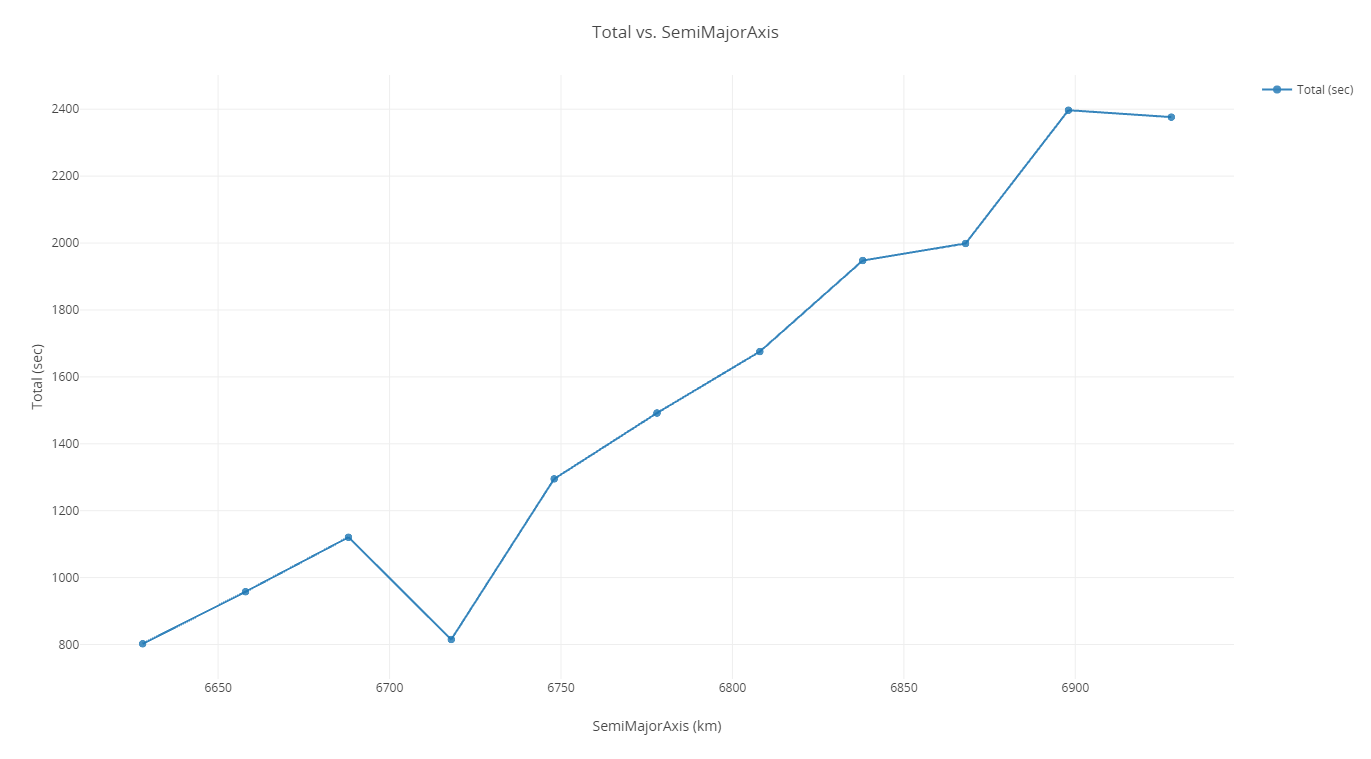
Circular orbit Total vs. SemiMajor Axis 2D Line Plot
You can see from your plot that there is a general trend of a longer total access duration with a higher semi-major axis. Keep this in mind as you perform further trade studies.
Performing an inclination Parametric Study
Now that you understand the relationship between the semi-major axis and total duration, explore the inclination. How will orbits with different inclinations affect the total observation time (total complete access duration)?
- Close the 2D Line Plot and the Table page when you are finished.
- Click when prompted to close your trade study without saving.
- Return to the Parametric Study tool.
- Click and drag Inclination () from the Component Tree to the Design Variable field.
- Set the following Design Variable parameters:
- Click .
This will replace SemiMajorAxis as the Design Variable.
| Option | Value |
|---|---|
| starting value | 30 |
| ending value | 90 |
| step size | 10 |
Later, you will perform another study with more refined values, but for now, use this range.
Visualizing the results with a 2D Line Plot
Create a 2D Line Plot to help you visualize the results of the inclination Parametric Study.
- Close the 2D Scatter Plot that opened when the trade study finished running.
- Click Add View () on the Table Page toolbar.
- Select 2D Line Plot () in the drop-down menu.
- Examine the results.
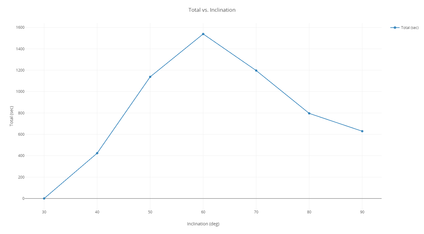
Circular orbit Total vs. Inclination 2D Line Plot
You can see from your plot that there is a peak between 50 and 70 degrees. You'll examine this further in the next section.
Closing out your trade study
Close out your trade study for the next section.
- Close the 2D Line Plot and the Table page when you are finished.
- Click when prompted to close your trade study without saving.
- Close the Parametric Study tool.
Analyzing the results with Carpet Plots
Now that you have performed the two individual variable Parametric Studies, you have an idea for the general ranges where the duration is the greatest for each orbital parameter variable (semi-major axis and inclination). These two parameters can be efficiently plotted together using a Carpet Plot to find the best combination that maximizes the total observation time duration. A Carpet Plot is a means of displaying data dependent on two variables in a format that makes interpretation easier than normal multiple curve plots. A Carpet Plot can be thought of as a multidimensional Parametric Study, except you now have two variables instead of one.
- Click Carpet Plot (
 ) on the Standard toolbar.
 - Click and drag SemiMajorAxis () from the Component Tree to the first Design Variables field when the Carpet Plot tool opens.
- Set the following SemiMajorAxis Design Variable values:
- Click and drag Inclination () from the Component Tree to the second Design Variable field.
- Set the following Inclination Design Variable values:
- Drag Total () from the Component Tree to the Responses field.
- Click .
| Option | Value |
|---|---|
| From | 6828 |
| To | 6928 |
| Num Steps | 5 |
These values reflect the best narrowed-down ranges from your semi-major axis Parametric Study.
| Option | From |
|---|---|
| From | 50 |
| To | 70 |
| Num Steps | 5 |
These values reflect the best narrowed-down ranges from your inclination Parametric Study.
Visualizing the results with a Contour Plot
Create a Contour Plot to help you visualize the results of the Carpet Plot study.
- Close the Carpet Plot that was automatically generated when the trade study finished running.
- Click Add View () on the Table Page toolbar.
- Select Contour Plot (
 ) in the drop-down menu to create a new plot.
 - Examine the results.
- Close the Contour Plot and the Table page when you are finished.
- Click when prompted to close your trade study without saving.
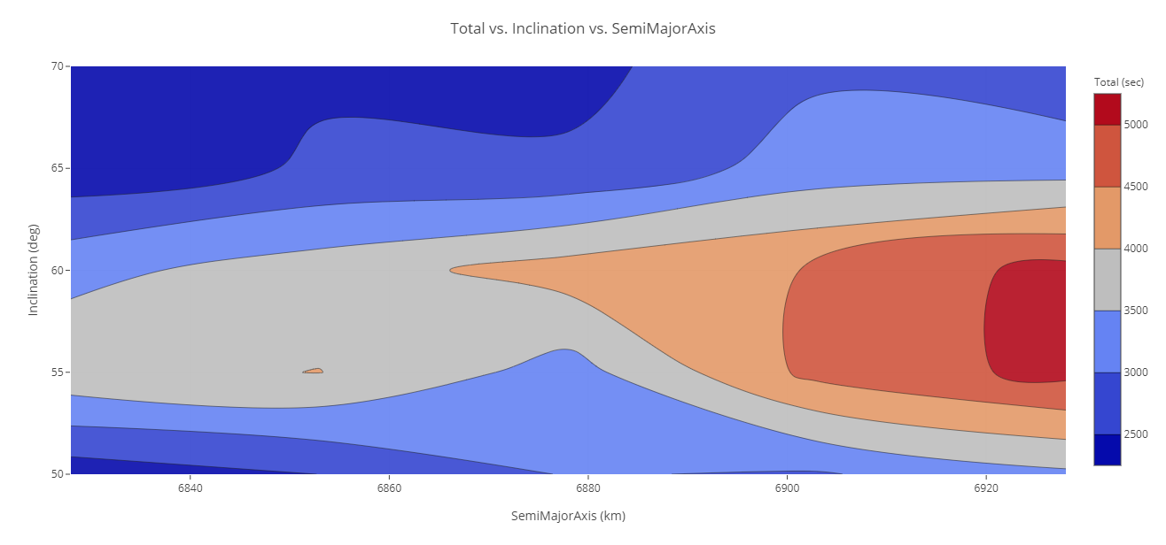
Circular orbit Total Vs. Inclination vs. SemiMajor Axis Contour Plot
Looking at the results from the Contour Plot, you can see that the ranges can be narrowed even further.
Refining and rerunning your Carpet Plot study
From the results of your Carpet Plot study, you can see that the bounds of your range can be narrowed down even further. Enter these new bounds and perform your Carpet Plot study again.
- Return to the Carpet Plot tool and update the From and To values:
- Click .
- Close the Carpet Plot that was automatically generated when the trade study finished running.
- Bring the Table page to the front when all runs are completed.
- Click Add View () on the Table Page toolbar.
- Select Contour Plot () in the drop-down menu.
- Close the Contour Plot and the Table page when you are finished.
- Click when prompted to close your trade study without saving.
| Name | From | To | Num Steps |
|---|---|---|---|
| SemiMajorAxis | 6900 | 6928 | 5 |
| Inclination | 50 | 60 | 5 |
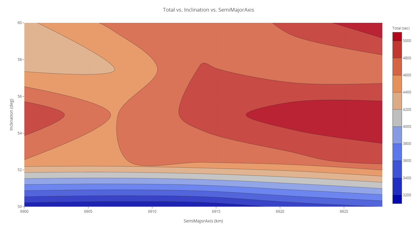
Updated circular orbit Total Vs. Inclination vs. SemiMajor Axis Contour Plot
From the plot, you can determine the best range of values for a circular orbit.
Performing eccentric orbit trade studies
You've studied STKSat in a circular orbit; now, analyze it in an elliptical orbit. Using the defined upper and lower orbital limits, 550 kilometers and 250 kilometers, the highest orbital eccentricity (e) you could possibly have is 0.0221. This comes from this formula:
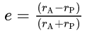
Where rA and rP are the radii of apogee and perigee, 6,928 kilometers and 6,628 kilometers, respectively. These values come from the radius of the Earth plus the minimum radius of perigee and the maximum radius of apogee, respectively.
To remain consistent with the radii of apogee and perigee, the semi-major axis must also be adjusted. The semi-major axis (a) can be calculated from the formula:
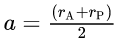
Thus, using the respective radii of apogee and perigee of 6,928 kilometers and 6,628 kilometers, the semi-major axis for that eccentricity is calculated to be 6,778 kilometers.
Adding additional input variables
To study an elliptical orbit, add the argument of perigee and the eccentricity as additional input variables.
- Right-click on the STK_ODTK13 component in the Analysis View.
- Select Show Component's GUI (
 ) in the shortcut menu.
 - Select STKSat () in the STK Variables tree when the STK Analyzer window opens.
- Expand () Propagator (J2Perturbation) () in the STK Property Variables tree.
- Select ArgOfPerigee ().
- Move () ArgOfPerigee () to the Analyzer Variables list.
- Select Eccentricity ().
- Move () Eccentricity () to the Analyzer Variables list.
- Click to confirm your selection and to close the STK Analyzer window.
Updating the values
With your variables added, update the values for your eccentricity trade studies.
- Expand () all the elements in the Component Tree.
- Click in the Value field for SemiMajorAxis.
- Enter 6778.
- Select the Enter key.
- Enter 0.0221 in the Eccentricity field.
- Select the Enter key.
- Save (
 ) your ModelCenter workflow.
Performing an inclination Parametric Study
Perform another Parametric Study to study the effects of the new orbital eccentricity.
- Click Parametric Study () in the Standard toolbar.
- Click and drag Inclination () from the Component Tree to the Design Variable field.
- Set the following Design Variable value:
- Drag Total () from the Component Tree to the Responses field.
- Click .
| Option | Value |
|---|---|
| starting value | 45 |
| ending value | 90 |
| number of samples | 11 |
Visualizing the results with a 2D Line Plot
Create a 2D Line Plot to help you visualize the results of the inclination Parametric Study.
- Close the 2D Scatter Plot that opened when the trade study finished running.
- Click Add View () on the Table Page toolbar.
- Select 2D Line Plot () in the drop-down menu.
- Examine the results.
- Close the 2D Line Plot the Table page when you are finished.
- Click when prompted to close your trade study without saving.
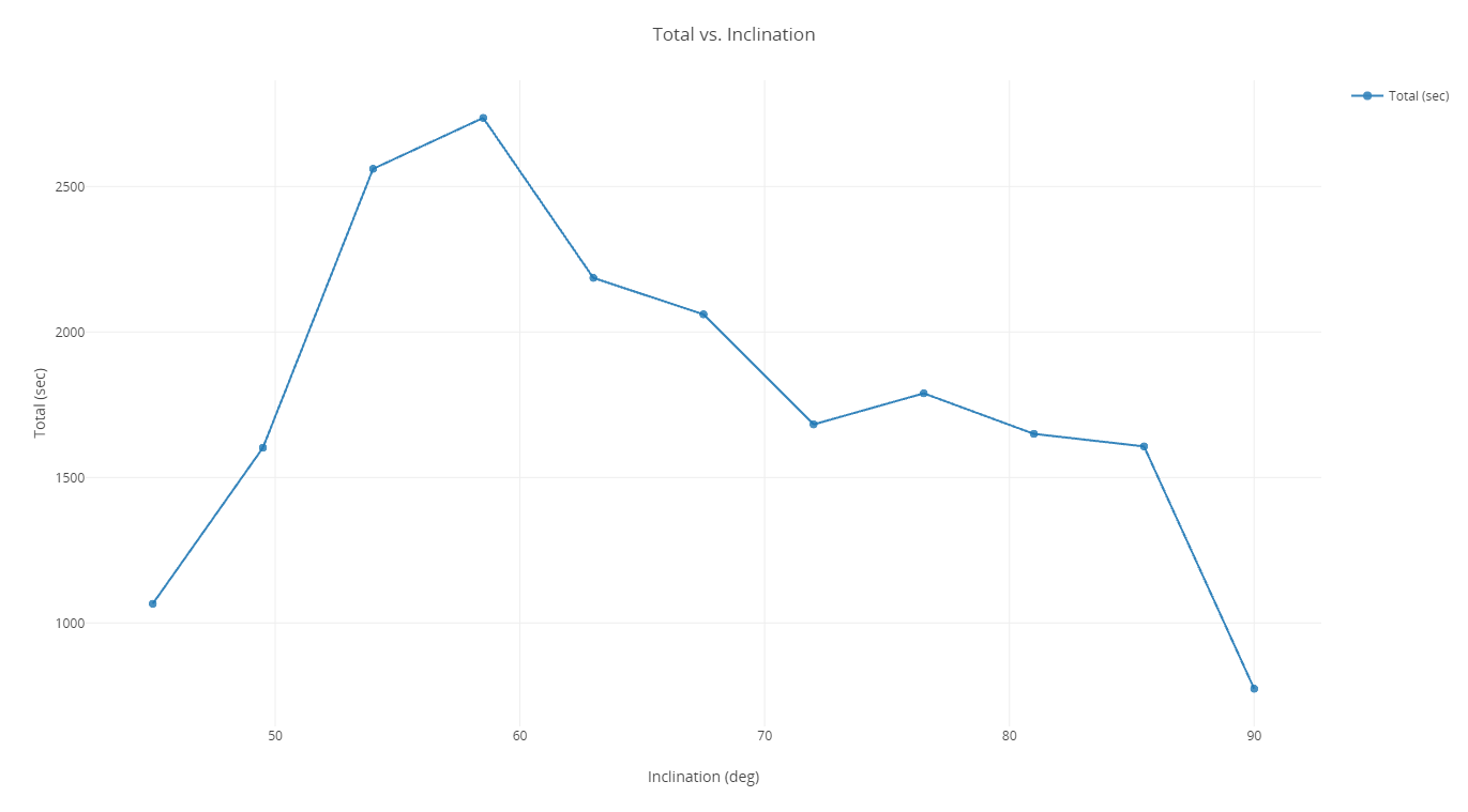
Elliptical orbit Total vs. Inclination 2D Line Plot
From these results, you can conclude an appropriate inclination range is 50 to 65 degrees.
Performing an argument of perigee Parametric Study
Examine the affects of changing the argument of perigee on the total duration.
- Return to the Parametric Study tool.
- Click and drag ArgOfPerigee () from the Component Tree to the Design Variable field.
- Set the following Design Variable values:
- Click .
| Option | Value |
|---|---|
| starting value | 0 |
| ending value | 360 |
| number of samples | 10 |
Visualizing the results with a 2D Line Plot
Create a 2D Line Plot to help you visualize the results of the argument of perigee Parametric Study.
- Close the 2D Scatter Plot that opened when the trade study finished running.
- Click Add View () on the Table Page toolbar.
- Select 2D Line Plot () in the drop-down menu.
- Examine the results.
- Close the 2D Line Plot the Table page when you are finished.
- Click when prompted to close your trade study without saving.
- Close the Parametric Study tool.
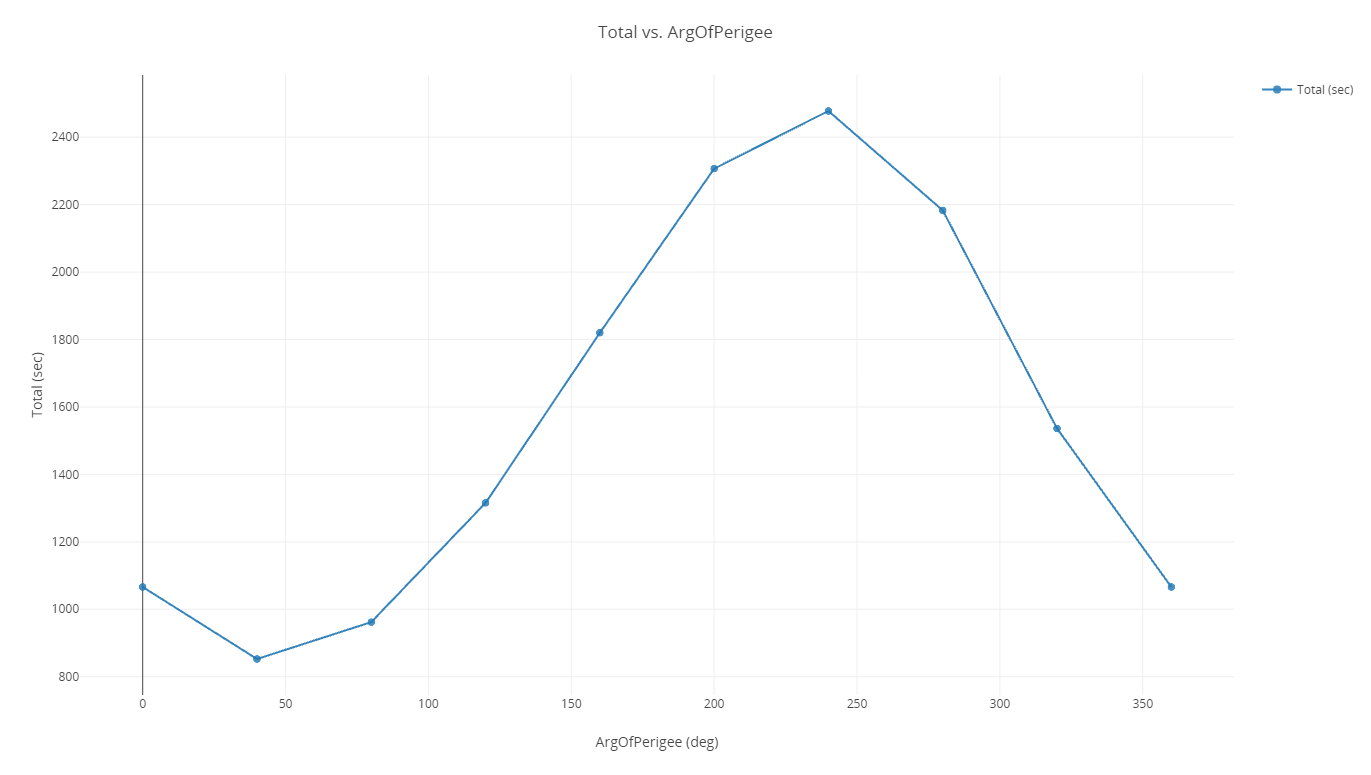
Elliptical orbit Total vs. Argument of perigee 2D Line Plot
You can see that a good range for the argument of perigee from this study is 200 to 300 degrees.
Generating a Carpet Plot
Now that you have performed Parametric Studies on each parameter, you have an idea for the general ranges where the duration is the greatest for each orbital parameter variable (semi-major axis and inclination). These two parameters can be plotted together efficiently to find the best combination that maximizes.
- Click Carpet Plot () on the Standard toolbar.
- Drag ArgOfPerigee () from the Component Tree to the first Design Variable field.
- Drag and Inclination () from the Component Tree to the second Design Variable field.
- Enter the following parameters, as concluded from your Parametric Studies:
- Drag Total () from the Component Tree into the Responses field.
- Click .
| Name | From | To | Num Steps |
|---|---|---|---|
| ArgOfPerigee | 200 | 300 | 6 |
| Inclination | 50 | 65 | 6 |
Visualizing the results with a Contour Plot
Create a Contour Plot to help you visualize the results of the Carpet Plot study.
- Close the Carpet Plot that was automatically generated when the trade study finished running.
- Click Add View () on the Table Page toolbar.
- Select Contour Plot () in the drop-down menu.
Increasing the number of contours
Increase the number of contours on the plot to better understand the data.
- Click Series in the Plot Options menu when the Contour Plot opens.
- Select All series (contour) in the Series drop-down menu.
- Select the Range/bins tab.
- Increase the Contours ... Max # to 20.
- Click anywhere on the Contour Plot to close the Plot Options menu.
- Review the Contour Plot.
- Close the Contour Plot and the Table page when you are finished.
- Click when prompted to close your trade study without saving.
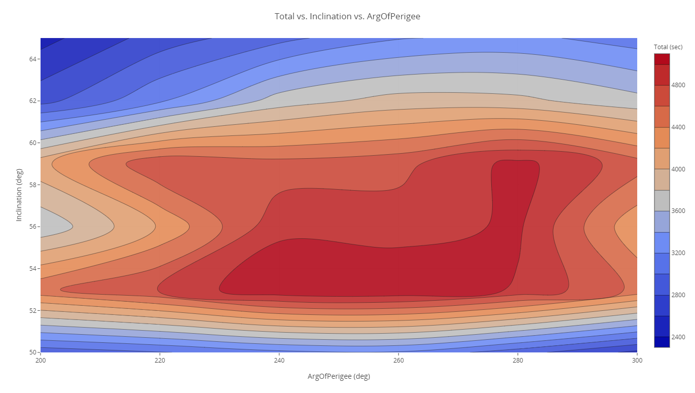
Elliptical orbit Total vs. Inclination vs. Argument of perigee Contour Plot
You can see from your plot that you can considerably narrow your ranges of values to study.
Refining your Carpet Plot
From the results of your previous Carpet Plot study, you can see there is a high total duration somewhere around an argument of perigee of 260 and an inclination of 53 degrees. Narrow the bounds and run your Carpet Plot study again.
- Return to the Carpet Plot tool and update the From and To values:
- Click .
- Close the Carpet Plot that was automatically generated when the trade study finished running.
- Click Add View () on the Table Page toolbar.
- Select Contour Plot () in the drop-down menu.
| Name | From | To | Num Steps |
|---|---|---|---|
| ArgOfPerigee | 220 | 280 | 6 |
| Inclination | 50 | 60 | 6 |
Increasing the number of contours
As before, increase the number of contours on the plot to better understand the data.
- Click Series in the Plot Options menu when the Contour Plot opens.
- Select All series (contour) in the Series drop-down menu.
- Select the Range/bins tab.
- Increase the Contours ... Max # to 20.
- Click anywhere on the Contour Plot to close the Plot Options menu.
- Review the Contour Plot.
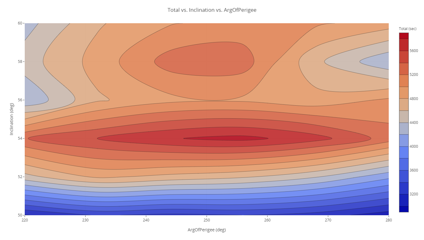
Updated Elliptical orbit Total vs. Inclination vs. Argument of perigee Contour Plot
From these results, the orbit with the greatest total coverage duration with an eccentricity of 0.0221 and a semi-major axis of 6,778 kilometers would have an inclination of 54 degrees and an argument of perigee of about 255 degrees.
Saving your model
Save your work and close out ModelCenter application.
- Close out any open plots, tools, and the Data Explorer window.
- Click when prompted to close your trade study without saving.
- Click Save () to save your ModelCenter workflow.
- Close the ModelCenter application.
Updating STKSat's orbit
Now that you have determined the optimal elliptical orbital for your scenario, update STKSat's orbital parameters with these new values.
- Reopen the STK application ().
- Reopen the SatOrbitDesignStarter scenario.
- Open STKSat's () Properties ().
- Select the Basic - Orbit page.
- Enter the optimal values you determined by performing your trade studies:
- Click to confirm your changes and to close the Properties Browser.
| Parameter | Value |
|---|---|
| Semimajor Axis | 6778 km |
| Eccentricity | 0.0221 |
| Inclination | 54 deg |
| Argument of Perigee | 255 deg |
Viewing STKSat's orbit
Once you have updated the orbital parameters, examine your changes in the 3D Graphics window.
- Bring the 3D Graphics window to the front.
- Right-click on STKSat () in the object browser.
- Select Zoom To in the shortcut menu.
- Use your mouse to get a good view of STKSat's orbit.
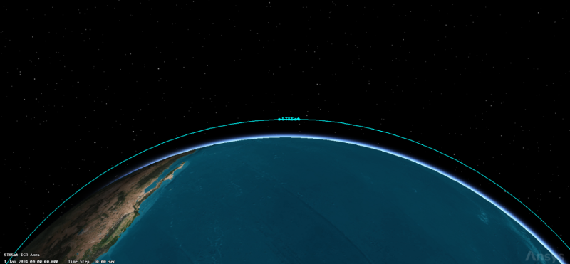
Propagated elliptical orbit of STKSat
Saving your work
Clean up your workspace and close out your scenario to prepare for the next lesson in the Space Mission Analysis and Design series.
- Close all reports and windows except the 2D and 3D Graphics windows.
- Save () your work.
- Close the scenario when you are finished.
Summary
In this tutorial you created an access between a satellite's imaging camera and a constellation of volcanoes. Using the ModelCenter software and the STK Plugin for ModelCenter, you optimized its orbit. First, using parametric trade studies, you determined that a higher semi-major axis resulted in longer access periods. With that in mind, you then conducted trade studies for an eccentric orbit to find the optimal orbital parameters for the maximum complete access duration.
Space Mission Analysis and Design Part 2: Solar and Power Design
The