STK Premium (Space) or STK Enterprise
You can obtain the necessary licenses for this tutorial by contacting AGI Support at support@agi.com or 1-800-924-7244.
Optional Product Install: This lesson uses the Ansys Discovery™ 3D product simulation software. You can obtain a license for this product by contacting AGI Support at support@agi.com or 1-800-924-7244.
Optional Utility Install: This lesson uses the Discovery STK Model Add-in. You can download the utility from the web at
This lesson requires STK 13.0 or newer to complete in its entirety. If you have an earlier version of the STK software, you can view a legacy version of this lesson.
The results of the tutorial may vary depending on the user settings and data enabled (online operations, terrain server, dynamic Earth data, etc.). It is acceptable to have different results.
Capabilities covered
This lesson covers the following capabilities of the Ansys Systems Tool Kit® (STK®) digital mission engineering software:
- STK Pro
- Analysis Workbench
- STK SatPro
Problem statement
Engineers and operators want to design a mission to characterize the steam, ash, and lava emissions of active volcanoes in the United States. The objective of the satellite, STKSat, is to image these volcanoes to provide early indications of volcanic eruption and to transmit the images to a ground site for analysis. The satellite's electrical power system (EPS) will include large, deployable solar panels and a battery, which will supply power to the other subsystems on board the satellite as needed. They want to determine what combination of solar panel system and battery from the available options will best satisfy the mission requirements.
The mission requirements for the EPS are as follows:
- The solar panel-battery combination must be able to supply at least 0.75 W of power to STKSat while it’s in a holding state.
- The solar panel-battery combination must be able to supply at least 6.0 W of power to STKSat while it’s transmitting data to the ground site.
- The solar panel-battery combination must be able to supply at least 3.25 W of power to the imaging camera and reaction wheels when the satellite is imaging a volcano.
- The battery must never fall below its rated depth of discharge (DoD).
Differences in weight between the components will not be taken into account, since they are minimal.
Solution
Use the STK software's Solar Panel tool and the Analysis Workbench capability to approach this study in three stages:
- In the first stage, you will use a model of STKSat and the STK SatPro capability's Solar Panel tool determine when over the course of a year the satellite's solar panels will generate the most and least amount of power.
- In the second stage, you will use the Analysis Workbench capability to gather power consumption data during the period having the longest duration of data transmission to the ground site while the solar panels are receiving the least amount of sunlight. This will be the period that has little or no power generation from the solar panels and the greatest power draw on the battery, producing its maximum expected DoD.
- In the third and final stage, you will analyze your findings to determine the least expensive combination of solar panel system and battery for the satellite's EPS that meets the mission requirements.
What you will learn
Upon completion of this tutorial, you will be able to:
- Load satellite models registered for solar panel analysis into the STK application
- Gather solar power generation data from a model satellite using the Solar Panel tool
- Use the Analysis Workbench capability to model spacecraft power consumption
Video guidance
Watch the following video. Then follow the steps below, which incorporate the systems and missions you work on (sample inputs provided).
Using the starter scenario
The starter scenario contains the constellation of volcanoes to be studied, the satellite, its imaging camera, and a Chain object analytically linking the constellation to the camera. Additionally, it includes a Discovery geometry file, two model files, and a Microsoft Excel workbook.
Downloading the starter VDF
Download the zipped starter VDF file.
- Download the zipped folder here: https://support.agi.com/download/?type=training&dir=sdf/help&file=SolarPowerDesignStarter_v13.zip
- Navigate to the downloaded folder.
- Right-click on SolarPowerDesignStarter_v13.zip.
- Select Extract All... in the shortcut menu.
- Set the Files will be extracted to this folder: path to the location of your choice. The default path is C:\Users\<username>\Downloads\SolarPowerDesignStarter_v13.
- Click .
- Go to the chosen folder.
- SolarPowerDesignStarter.vdf will be in the extracted folder.
If you are not already logged in, you will be prompted to log in to agi.com to download the file. If you do not have an agi.com account, you will need to create one. The user approval process can take up to three (3) business days. Please contact support@agi.com if you need access sooner.
Opening the starter scenario
Now that you have extracted the starter VDF, open it in the STK application.
- Launch the STK (
 ) application.
 - Click
 Open a Scenario in the Welcome to STK dialog box.
 - Browse to location of your extracted VDF file.
- Select SolarPowerDesignStarter.vdf.
- Click .
Saving the VDF as a scenario
Save and extract the VDF data in the form of a scenario folder. When you save a VDF in the STK application, it will save in its originating format. That is, if you open a VDF, the default save format will be a VDF (.vdf). If you want to save and extract a VDF as a scenario folder, you must change the file format by using the Save As feature. This will create a permanent scenario file complete with child objects and any additional files packaged with the VDF.
- Open the File menu.
- Select Save As....
- Select the STK User folder in the navigation pane when the Save As dialog box opens.
- Select the SolarPowerDesignStarter folder.
- Click .
- Select Scenario Files (*.sc) in the Save as type drop-down list.
- Select the SolarPowerDesignStarter Scenario file in the file browser.
- Click .
- Click in the Confirm Save As dialog box to overwrite the existing scenario file in the folder and to save your scenario.
A scenario folder with the same name as the VDF was created for you when you opened the VDF in the STK application. This folder contains the temporarily unpacked files from the VDF.
The following non-STK files will be extracted to the SolarPowerDesignStarter folder:
- STKSatModelDsco.dsco
- STKSatModelDsco.glb
- STKSatModel.glb
- Final Power Analysis Blank.xlsx
When saving a VDF containing external files as a scenario folder, you must extract its contents to the scenario folder the STK application automatically creates for you in the STK User folder. This allows files packaged with the VDF, such as data files, reports, presentations, HTML pages, scripts, spreadsheets, and other files, to unpack to the scenario folder. If you save the VDF as a scenario folder in another location, these additional files will not be included. See the
Save (![]() ) often!
) often!
Updating the analysis period
Update your scenario's Start and Stop times for the next stages in the tutorial.
- Right-click on SolarPowerDesignStarter (
 ) in the Object Browser.
 - Select Properties (
 ) in the shortcut menu.
 - Select the Basic - Time page when the Properties Browser opens.
- Modify the start and stop times of your scenario to the values listed in the table below:
- Click to accept your changes and to close the Properties Browser.
| Field | Value |
|---|---|
| Start | 1 Jan 2024 00:00:00.000 UTCG |
| Stop | 1 Jan 2025 00:00:00.000 UTCG |
Adding a ground site
STKSat transmits data down to a ground site in Exton, Pennsylvania. Model the ground site with a Facility (![]() ) object. Later, you will compute access to it so that you can quantify the relationship between the satellite and the ground site. In Part 3 of this series, you will examine the communications link in more detail.
) object. Later, you will compute access to it so that you can quantify the relationship between the satellite and the ground site. In Part 3 of this series, you will examine the communications link in more detail.
- Insert a Facility (
 ) object using the Insert Default () method.
 - Rename Facility1 () Exton.
- Open Exton's () Properties ().
- Select the Basic – Position page.
- Make the following changes:
| Latitude | Longitude |
|---|---|
| 40.0388 deg | -75.6005 deg |
- Click .
- Right-click on Exton ().
- Select Zoom To in the shortcut menu.
Note the location of the Facility is in a field near the AGI Headquarters in Exton, Pennsylvania.
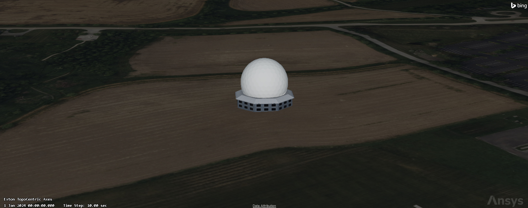
Exton ground site facility
The above image uses the Flashlight (![]() ) on the 3D Graphics toolbar to enhance visibility.
) on the 3D Graphics toolbar to enhance visibility.
Creating a solar array model with the Ansys Discovery software
Set the solar panel groups within a 3D object model of the satellite in a way that the STK application can register them using the Ansys Discovery™ 3D product simulation software. The SolarArray component includes the top faces of each set of solar panels in the 3D model, which will be used to create a solar panel group that includes all of the solar panels on the model
If you do not have access to the Discovery software, skip to the
The STKSatModelDsco.dsco file was created using version 2024R2 of the Ansys Discovery software. Because Discovery files are not backwards compatible, this lesson requires version 2024R2 of the Ansys Discovery software or newer to complete.
You must install the Discovery STK Model Add-in for use in the Discovery application to complete this section. Once the utility is installed, the main ribbon across the top of the Discovery application will show a tab called Systems Tool Kit (STK). Learn more about preparing CAD models for STK using the Discovery STK Model Add-in at
Loading the satellite geometry file into the Discovery Software
Open the STKSatModelDsco.dsco geometry file in the Discovery application.
- Open the Ansys Discovery application.
- Select Browse.
- Under Other Locations, select This PC.
- Navigate to the STKSatModelDsco.dsco file in your scenario folder.
- Double-click on the file open it.
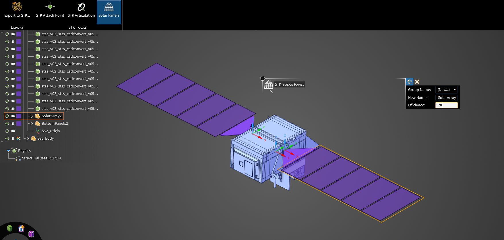
Configuring the solar panel arrays
Configure the model's solar panels for use in the STK application.
- Select the Systems Tool Kit (STK) window.
- Click .
- Select the SolarArray1 component, which is a child of SA1_Comp.
- Within the heads-up display, set the Group Name to (New...).
- Enter SolarArrays as the New Name.
- Change the Efficiency to 28.
- Select the SolarArray2 component, which is a child of SA2_Comp.
- Set the Group Name to SolarArrays to add it to the same group as SolarArray1.
Exporting the satellite model file from the Discovery application
Export the geometry file as a model that has solar panels registered for use with the STK software.
- Click .
- Ensure the Save as type is set to glTF Model for STK.
- Save your file as STKSatModelDsco.glb, if it does not already exist. Otherwise, choose a new name for your file.
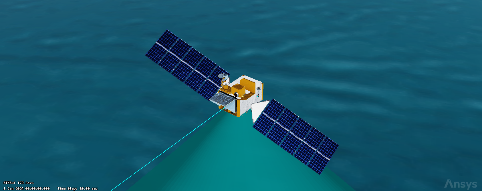
STKSAT Model in the ANsys Discovery Software
Updating STKSat's model in the STK application
Use a satellite model produced using the Ansys Discovery software that includes solar panels registered for analysis in the STK application. Later on, you will use the model to conduct a solar power analysis.
If you do not have access to the Ansys Discovery software, the file, STKSatModelDsco.glb, is supplied with the starter scenario.
Updating the model file
Load the STKSat Model in place of the default satellite model used in the STK application.
- Return to the STK application.
- Right-click on STKSat (
 ) in the Object Browser.
 - Select Properties () in the shortcut menu.
- Select the 3D Graphics - Model page.
- Click the Model File ellipsis (
 ).
). - Browse to the location of your STKSatModelDsco.glb file when the file dialog box opens.
- Select STKSatModelDsco.glb.
- Click to accept your change and to load the new model.
- Click to save your changes and to keep the Properties Browser open.
Rotating the STKSat model
Rotate the STKSat model in the scenario so that is oriented correctly for the analyses you'll be running in this series.
- Select the 3D Graphics - Offsets page.
- Select the Use check box in the Rotational Offset panel.
- Set the Y and Z values to 180 deg.
- Click to accept your changes and to close the Properties Browser.
Viewing STKSat's model
Once the 3D model has been updated and oriented correctly, examine the changes in the 3D Graphics window.
- Bring the 3D Graphics window to the front.
- Right-click on STKSat () in the object browser.
- Select Zoom To in the shortcut menu. You will notice the solar panels are accurately modeled. but the model itself however does not feature any graphic textures. The textures are not needed for this analysis.
- Click Start (
 ) on the Animation Toolbar to animate your scenario.
 - Watch as the solar panels track the Sun as STKSat orbits the earth.
- Click Reset (
 ) when finished.
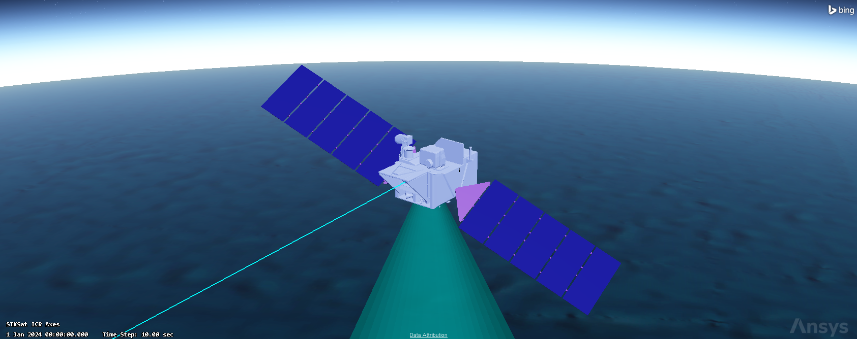
STKSat model created using the Ansys Discovery application
Performing power generation analysis
The SatPro capability extends the STK software into the realm of high-fidelity satellite systems modeling and analysis. SatPro provides you with a collection of satellite engineering tools, including the
You'll use the Solar Panel tool to analyze and view STKSat's solar panels. Due to Earth's elliptical orbit around the Sun, the Earth does not consistently receive solar rays of the same strength from month to month, or even day to day. The same concept applies to satellites. You will gather the solar panel data during the 15th day of each month, since analyzing the scenario over for an entire year is resource intensive and the data produced for this sample period can be extrapolated across the entire month.
Opening the Solar Panel tool
Open the Solar Panel tool for STKSat.
- Right-click on STKSat () in the Object Browser.
- Select Satellite in the shortcut menu.
- Select Solar Panel... in the Satellite submenu to open the Solar Panel tool interface.
- Arrange the display so you can see the Solar Panel and Solar Panel View windows at the same time.
The Solar Panel View window that displays the STKSat model is for visualizing the solar thermal storage systems as the tool is run.
Analyzing power generation in January
Set up the analysis to see how much power STKSat can generate in January. Rather than analyze the entire month, you will focus on power generated in the middle of the month; your assumption is that a measurement in the middle of month will reflect the total month. Additionally, by limiting the scope of the analysis, you can calculate the results faster.
- In the Solar Panel window, select SolarArrays in the Solar Panel Group list in the Visualization panel.
- Click in the Obscuring Objects panel to ensure no objects are being used for obscuration.
- Set the Time Step to 120 seconds in the Data panel.
- Change the Start Time to 15 Jan 2024 00:00:00.000 UTCG.
- Change the Stop Time to 16 Jan 2024 00:00:00.000 UTCG.
- Click .
- Click on any dialog boxes that may appear to allow the tool to run.
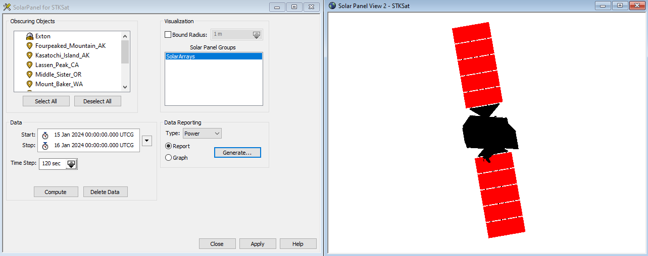
Solar Panel tool for and solar panel view of STKSat
Once the tool has collected all its data, the STKSat model in the Solar Panel View window will stop rotating.
Examining the Solar Panel Power report
When the calculation is complete, you can generate a report of the Solar Panel Power results.
- Ensure the Type in the Data Reporting panel is set to Power
- Ensure that Report option is selected.
- Click .
- Set the Jump: option to All Solar Panel Group to jump to that section in the report when the Solar Panel Power report appears.
- Examine the results.
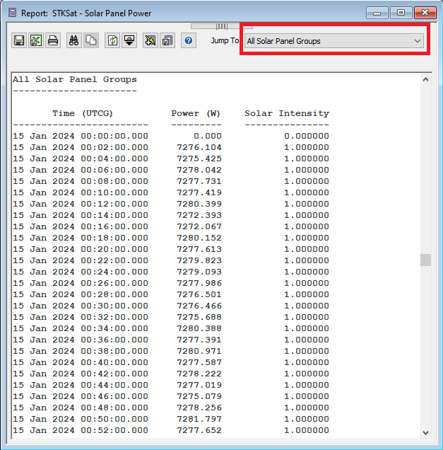
STKSat - Solar Panel Power report for January
Exporting the Solar Panel Power report to Microsoft Excel
Now that you have generated the solar panel power data for January, export this report for future analysis.
- In the Report window, click Save as .csv (
 ).
). - Navigate to your desired save location and rename the CSV to January.
- Click .
- Close the Report window.
- Open January.csv in Excel.
- Delete all the rows before the All Solar Panel Groups section. The only remaining data should be for the All Solar Panel Groups.
- Highlight the rows.
- Right-click on your selection.
- Select Delete... in the shortcut menu
- Select Entire row in the Delete dialog box.
- Click inside cell E1.
- Enter the formula
=SUM(B:B). - Save the CSV with your changes.
The above command allows Excel to sum the power generation data for each time step and report the total power generation. However, copying and pasting the total power generation value may result in an error.
Generating monthly data for February through December
You generated the data just for the month of January. Repeat the steps above to generate reports for the remaining year. Please note that the unit for months uses its three-letter designation, for example, Sep denoting September.
- Bring the STK application to the front.
- Click in the Data panel of the Solar Panel window.
- Repeat the steps from Examining the Solar Panel Power report and Exporting the Solar Panel Power report to Microsoft Excel for each of the remaining months in the year, changing the Start and Stop Times to the 15th and 16th of each month, respectively, and being sure to delete the data between each run.
- Close the Report, Solar Panel View, and Solar Panel windows once each month's power report has been generated.
Comparing solar power generation over one year
Sum up the All Solar Panel Groups data for each month within the Excel files and create a separate file to summarize the results for comparison.
- Create a new Excel spreadsheet.
- Save the new spreadsheet as Solar Power Year Summary.
- Create 3 columns with the following headings:
- Month
- Number (#)
- Power (W)
- Enter in the name and corresponding number for each month (January - December).
- Open the twelve CSV files for January through December.
- Copy and paste the power values in each cell E1 into the Power (W) column of the Solar Power Year Summary spreadsheet for the corresponding month.
- Enter the total power value.
- Highlight the Number (#) and Power (W) columns in the Solar Power Year Summary to generate a Scatter with Smooth Lines and Markers plot.
- Format the chart as desired.
- Observe how STKSat generates power over the course of one year.
A satellite's orbital parameters affect how the solar power generation varies over the year. A satellite with different orbital parameters wouldn't necessarily show the same trend as STKSat in this scenario.
Analyzing power consumption / power generation data
The most important requirement for solar and power design is to ensure the satellite constantly has enough power to perform all of its functions. You want to design an electrical power system that can sustain the satellite during the time when it is generating the least amount of power.
You will further analyze the month that generated the least amount of power in order to determine the longest access interval between STKSat and Exton that is in either in penumbra or umbra. Assume that STKSat's transmitter and receiver will be active during the entire interval, meaning that STKSat will experience a lengthened period of power draw while operating during the month that it receives the least amount of power generation from sunlight. The power draw from the camera will be accounted for but it is not the main focus, since it draws much less power than the transmitter.
Determining penumbra / umbra access times and maximum access duration
In this section, you will shorten your Scenario Interval, since you are only interested in the month that STKSat generates the least amount of power. The reported access times will be generated for STKSat (![]() ) whenever it is either in the penumbra or umbra of earth's shadow.
) whenever it is either in the penumbra or umbra of earth's shadow.
- Right-click on SolarPowerDesignStarter () in the Object Browser.
- Select Properties () in the shortcut menu.
- Select the Basic - Time page.
- In the Analysis Period panel, set the Start Time to be the first of the month determined above with a time of 00:00:00.000 UTCG
- Set the Stop Time to be the first of the following month with a time of 00:00:00.000 UTCG.
- Click to set the scenario analysis interval and to close the Properties Browser.
- In the Animation toolbar, click Reset (
 ) when finished.
Make sure the start year is 2024 and the stop year fits accordingly. An example of the Scenario Interval for June being the month with least power generation is shown below.
| Option | Value |
|---|---|
| Start Time | 1 Jun 2024 00:00:00.000 UTCG |
| Stop Time | 1 Jul 2024 00:00:00.000 UTCG |
Adding lighting constraints to STKSat
Use lighting constraints to limit your analysis to when STKSat is within earth's penumbra or umbra.
Adding lighting constraints in versions 12.9 and later of the STK software
Add a lighting constraint to STKSat on the Constraints - Active page when using versions 12.9 and later of the STK software.
- Right-click on STKSat () in the Object Browser.
- Select Properties () in the shortcut menu.
- On the Constraints - Active page, click Add new constraints (
 ).
). - Select Lighting from the Constraint Name list.
- Click .
- Click .
- Select Penumbra or Umbra from the Lighting drop-down list in Constraint Properties section.
- Click .
Adding lighting constraints in Version 12.8 and Earlier of the STK Software
Add a lighting constraint to STKSat on the Constraints - Lighting page when using versions of the STK software that are older than version 12.9.
- Right-click on STKSat () in the Object Browser.
- Select Properties () in the shortcut menu.
- On the Constraints – Sun page, select the check box for Lighting.
- Select Penumbra or Umbra from the drop-down list.
- Click .
Computing access during the largest power draws
You need to figure out if the solar panels and batteries can supply enough power to transmit the data when they are generating the least amount of power; that is, when the satellite is within earth's shadow. In the previous step, you set a lighting condition; this will limit access times to when the satellite is in the earth's penumbra or umbra. In this section, you will compute that access. You know that the satellite will be transmitting data to the ground site, and that is when it will have the largest power draw. Your access calculation will be a placeholder for this draw.
- Right-click on STKSat () in the Object Browser.
- Select Access... (
 ) in the shortcut menu.
 - Ensure the top of the window says Access for: STKSat ().
- Select Exton () in the Associated Objects list and click
 .
. - In the Reports panel, click .
- Under Statistics at the bottom of the report, take note of the Start and Stop Times for the Max Duration of Access.
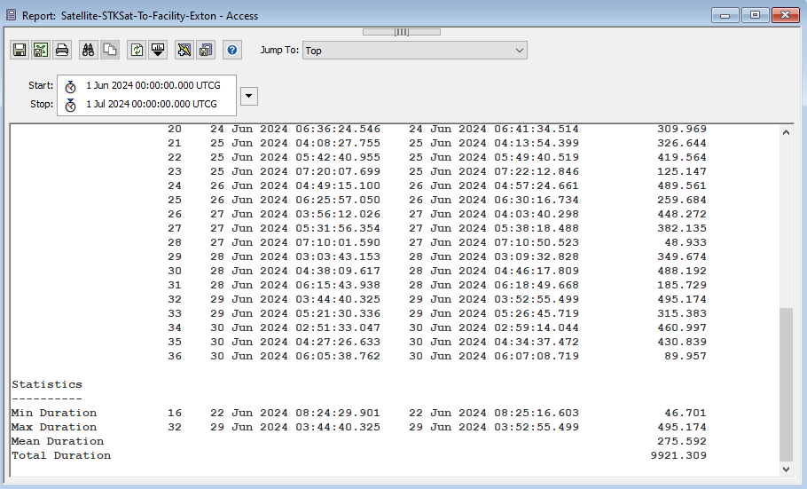
Satellite-STKSat-to-Facility-Exton Access report
Calculating total power generation
Analyze a brief Scenario Interval around the Start and Stop Times of STKSat's (![]() ) longest access duration while in penumbra or umbra. The Analysis Period of the Scenario will be shortened.
) longest access duration while in penumbra or umbra. The Analysis Period of the Scenario will be shortened.
- Right-click on SolarPowerDesignStarter () in the Object Browser.
- Select Properties () in the shortcut menu.
- In the Analysis Period panel, set the Start Time to be 24 hours before the start time of the longest access duration.
- Set the Stop time to be 24 hours after the Stop Time of the longest access duration.
- Click .
- In the Animation toolbar, click Reset () when finished.
- Close the Access Report.
Note: An example of the Scenario Interval for June's longest access duration being altered by 24 hours for the Start and Stop Times is shown below.
| Time Component | Start Time | Stop Time |
|---|---|---|
| Longest Access Duration | 29 Jun 2024 03:44:40.325 | 29 Jun 2024 03:52:55.499 |
| Scenario Analysis Period | 28 Jun 2024 03:44:40.325 | 30 Jun 2024 03:52:55.499 |
Calculating power generation during periods of penumbra and / or umbra
In the next sections, you'll calculate the power generated over the new scenario analysis period. Reopen the Solar Power interface to get started.
- Right-click on STKSat () in the Object Browser.
- Select Satellite in the shortcut menu.
- Select Solar Panel... in the Satellite submenu.
- Arrange the display so you can see the Solar Panel and the Solar Panel View windows at the same time.
Setting up and computing the power generation analysis
Now that the scenario time has been updated to reflect the 24 hours before and after the longest access / transmission window, generate a solar power report. You will use the updated scenario time for this solar power generation report.
- Click the down arrow (
 ) next to the Interval field in the Data panel.
 - Select Use Scenario Interval in the drop-down list.
- Select SolarArrays in the Solar Pane Groups list in the Visualization panel.
- Click in the Obscuring Objects panel to ensure no objects are being used for obscuration.
- Set the Time Step to 60 seconds.
- Click .
- Click on any dialog boxes that appear to allow the tool to run.
Examining the Solar Panel Power report
When the calculation is complete, you can generate a Solar Panel Power report to view the results.
- Ensure Type in the Data Reporting panel is set to Power and that the Report option is selected.
- Click the .
- Select All Solar Panel Groups in the Jump To drop-down list to jump to that section in the report.
- Examine the results.
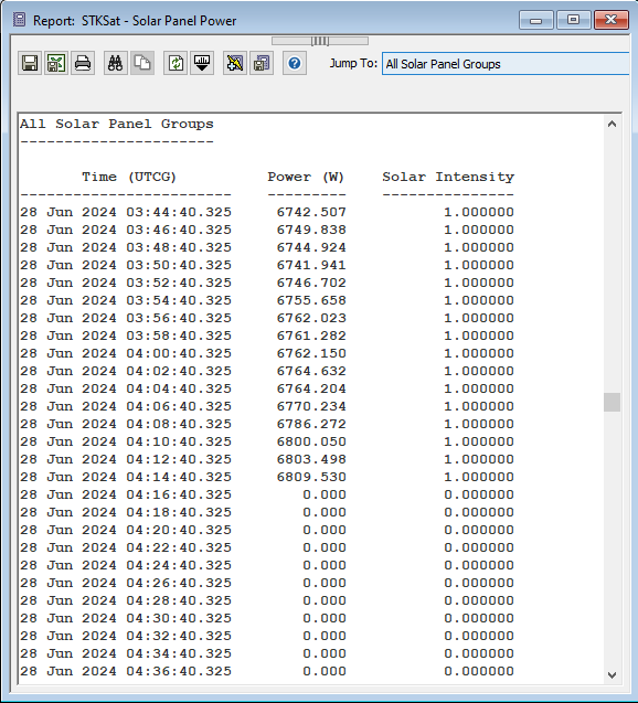
Solar panel power report for the focused scenario period
Exporting the report
Now that you have generated the solar panel power data for your focused scenario period, export the report for further analysis.
- In the Report window, click Save as .csv ().
- Navigate to your desired save location.
- Rename the file Total Power Generation.
- Click .
- Close the Report, Solar Panel View, and Solar Panel windows.
- Open the Total Power Generation file in Excel.
- Delete all the rows until the All Solar Panel Groups section. The only remaining data should be for the All Solar Panel Groups.
- Save the CSV file.
Calculating total power consumption
Use the Analysis Workbench capability to compute the total power consumption of STKSat over the detailed interval defined in the previous section. The total power consumed is a calculation of the variable power consumption of the satellite's on-board subsystems and the subsystems which constantly draw power. Since power production is recorded as positive values, all power consumption components are defined in negative values.
Calculating subsystem variable power consumption
STKSat contains several subsystems that allow the satellite to image the volcanoes and transmit the data. It is important to note that these subsystems have a variable power draw: they only draw power when they are turned on. The variable power draw values defined below can be combined in a series of scalar calculations to determine the power consumption of the subsystems during their use over the analysis period:
Variable Power Subsystems
| Subsystem | Power Draw (W) |
|---|---|
| Reaction Wheels | 3 (In use) |
| 0 (Off) | |
| Camera | 0.250 (In use) |
| 0 (Off) | |
| Transmitter | 6 (In use) |
| 0 (Off) |
Calculating access times
Before calculating the camera consumption, you must determine the times when the camera is active and imaging volcanoes. To do this, you can calculate complete Chain access using the Observe Chain (![]() ) object, which analytically links the camera to the constellation of volcanoes. The complete Chain access intervals will be used to calculate the imaging camera's power consumption over the scenario interval. The assumption is that the reaction wheels within the above table are being used when STKSat is able to image a volcano; their 3-Watt power draw allows STKSat to rotate in order to keep the camera pointed at the volcano.
) object, which analytically links the camera to the constellation of volcanoes. The complete Chain access intervals will be used to calculate the imaging camera's power consumption over the scenario interval. The assumption is that the reaction wheels within the above table are being used when STKSat is able to image a volcano; their 3-Watt power draw allows STKSat to rotate in order to keep the camera pointed at the volcano.
Computing Chain accesses
Compute the accesses for the Chain before building a report on the access times.
- Right-click on Observe (
 ) in the Object Browser.
 - Select Chain in the shortcut menu.
- Select Compute Accesses in the Chain submenu.
Generating a Complete Chain Access Report
Generate a
- Right-click on Observe ()in the Object Browser.
- Select Report & Graph Manager... (
 ) in the shortcut menu.
 - Select Observe () in the Object Type: Chain list.
- Expand (
 ) the Installed Styles folder (
 ) in the Styles list.
 - Select Complete Chain Access (
 ).
). - Click .
- Examine the results.
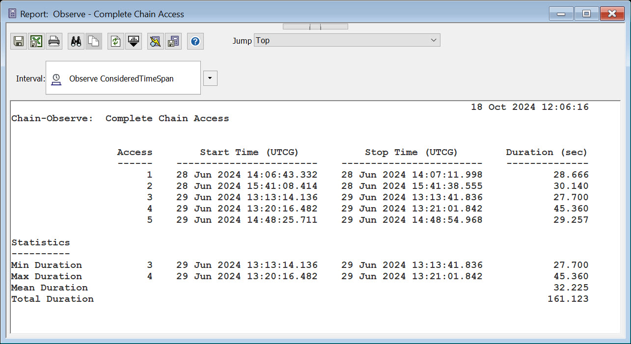
Complete Chain Access report
Updating the lighting constraint
Recall that earlier, you set a lighting constraint on STKSat. You need to clear STKSat’s lighting constraints back so that the access times are not restricted to only penumbra or umbra.
Removing lighting constraints in versions 12.9 and later of the STK software
Clear the lighting constraint from STKSat on the Constraints - Active page when using versions 12.9 and later of the STK software.
- Right-click on STKSat () in the Object Browser.
- Select Properties () in the shortcut menu.
- Select the Constraints - Active tab.
- Clear the Enable check box for Lighting.
- Click .
Removing lighting constraints in Versions 12.8 and Earlier of the STK Software
Clear the lighting constraint from STKSat on the Constraints - Lighting page when using versions of the STK software that are older than version 12.9.
- Right-click on STKSat () in the Object Browser.
- Select Properties () in the shortcut menu.
- Select the Constraints – Sun page.
- Clear the Enable check box for Lighting.
- Click to close the Properties Browser.
Defining the camera's power consumption
Use the Analysis Workbench capability to calculate the power the camera consumes when it is taking pictures of the volcanoes. The first step is to create a scalar calculation.
- Select Analysis Workbench... (
 ) from the Analysis menu.
 - Select the Calculation tab when the Analysis Workbench () opens.
- Select STKSat () in the object tree.
- Click Create new Scalar Calculation (
 ).
). - Click Type: when the Add Calculation Component dialog box opens.
- Select Constant () in the Select Component Type list when the Select Component Type dialog box opens.
- Click to set the calculation type and to close the Select Component Type dialog box.
- Enter Camera_Consumption in the Name field.
- Set the Constant Value field to -3.25 and leave the Dimension as Unitless.
- Click .
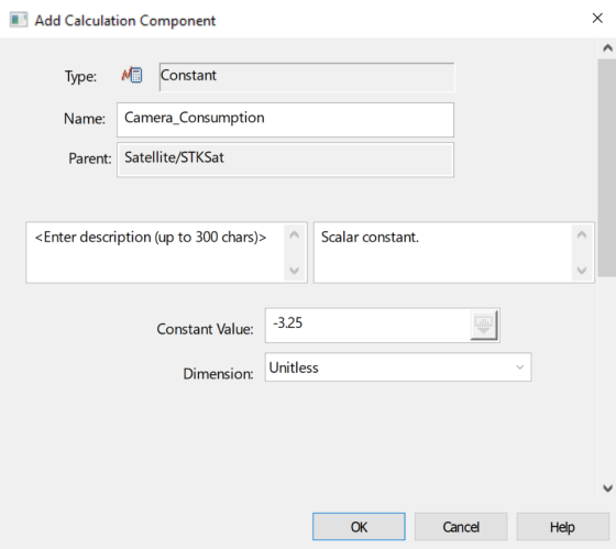
Camera Consumption scalar component
Calculating camera power consumption during image capture
You only want to calculate this power draw when the imaging camera is being used, which is when it is taking pictures of the volcanoes. Set up another Scalar Calculation to do this.
- Click Create new Scalar Calculation ().
- Click Type: when the Add Calculation Component dialog box opens.
- Select Integral in the Select Component Type list when the Select Component Type dialog box opens.
- Click to close the Select Component Type dialog box.
- Enter Camera_Consumption_Calc in the Name field.
- Set the Input Scalar to the Camera_Consumption:
- Click the Input Scalar ellipsis ().
- Select Camera_Consumption () in the My Components () folder in the in the Scalar Calculations for: STKSat list when the Select Reference Scalar Calculation dialog box opens.
- Click to close the Select Reference Scalar Calculation dialog box.
- Click the Input Scalar ellipsis (
- Select Cumulative to Current in the Accumulation Type drop-down list.
- Set the time limits to the access intervals defined in the Complete Chain Access Report:
- Click .
- Click the Time Limits ellipsis () when the Advanced Data dialog box opens.
- Select Observe () in the object tree.
- Select the CompleteChainAccessIntervals (
 ) component in the Components for: Observe list.
 - Click to close the Select Interval or List dialog box.
- Click twice to close the Advanced Data and Add Calculation Components dialog boxes and to keep the Analysis Workbench open.
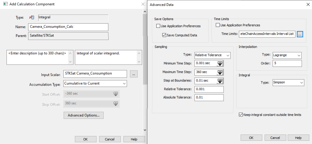
Camera power consumption scalar components
Defining the transmitter's power consumption
Use the Analysis Workbench capability to calculate the power the transmitter consumes when it is sending data to the ground site. The first step is to create a scalar calculation.
- Select the Calculation tab in Analysis Workbench ().
- Select STKSat () in the object tree.
- Click Create new Scalar Calculation ().
- Click Type: when the Add Calculation Component dialog box opens.
- Select Constant () in the Select Component Type list when the Select Component Type dialog box opens.
- Enter Transmitter_Consumption in the Name field.
- Set the Constant Value to -6 and leave the Dimension Unitless.
- Click .
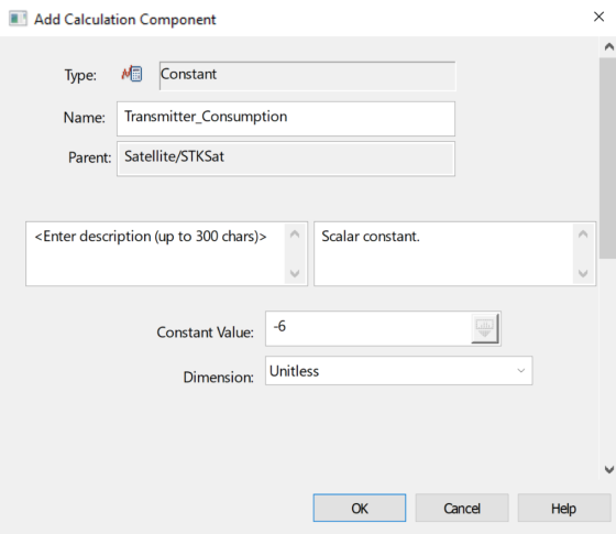
Transmitter Consumption scalar Calculation component
Calculating transmitter power consumption when sending data
You only want to calculate the power draw when STKSat has line-of-sight access to Exton; this represents when it is transmitting data. Set up another Scalar Calculation to do this.
- Select STKSat () in the object tree.
- Click Create new Scalar Calculation ().
- Click Type: when the Add Calculation Component dialog box opens.
- Click .
- Select Integral () in the Select Component Type list when the Select Component Type dialog box opens.
- Enter Transmitter_Consumption_Calc in the Name field.
- Set the Input Scalar to the Transmitter_Consumption scalar calculation:
- Click the Input Scalar ellipsis ().
- Select Transmitter_Consumption () in the My Components () folder in the Scalar Calculations for: STKSat list when the Select Reference Scalar Calculation opens.
- Click .
- Click the Input Scalar ellipsis (
- Set the Accumulation Type to Cumulative to Current.
- Set the time limits to use the access intervals between STKSat and Exton:
- Click .
- Click the Time Limits ellipsis ().
- Select Satellite-STKSat-To-Facility-Exton (
 ) in the object tree.
 - Select the AccessIntervals () component in the Components for: Satellite-Satellite-STKSat-To-Facility-Exton list.
- Click three times to create the new Scalar Calculation and keep the Analysis Workbench open.
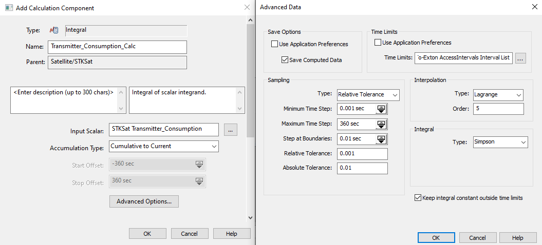
Transmitter power consumption scalar calculation components
Calculating combined variable power consumption
Combine the Camera Consumption Calculation and Transmitter Consumption Calculations to give the total variable power consumption. This will tell you how much power both subsystems will draw when the imaging camera is taking pictures and when the transmitter is transmitting.
- Select STKSat () in the object tree.
- Click Create new Scalar Calculation ().
- Click Type: when the Add Calculation Component dialog box opens.
- Select Function(x,y) () in the Select Component Type list when the Select Component Type dialog box opens.
- Enter Variable_Consumption_Function in the Name field.
- Leave the default Function a*x+b*y.
- Set Camera_Consumption_Calc Scalar Calculation () as the x reference scalar calculation:
- In the Arguments panel, click the x ellipsis ().
- Select Camera_Consumption_Calc () in the Scalar Calculations for: STKSat list.
- Click .
- In the Arguments panel, click the x ellipsis (
- Set Transmitter_Consumption_Calc Scalar Calculation as the y reference scalar calculation.
- In the Arguments panel, click the y ellipsis ().
- Select Transmitter_Consumption_Calc () in the Scalar Calculations for: STKSat list.
- Click .
- In the Arguments panel, click the y ellipsis (
- Leave all other values as their defaults.
- Click .

Variable power consumption scalar component
Defining constant power consumption
STKSat is constantly using power for its on-board computer and the receiver. Group the total constant value in a Scalar Calculation. The constant power consumption values defined below can be summed together in a single constant value component:
Constant Power Consumption Values
| Subsystem | Power (W) |
|---|---|
| Spacecraft Computer | 0.50 |
| Receiver | 0.25 |
- Select STKSat () in the object tree.
- Click Create new Scalar Calculation ().
- Click Type: when the Add Calculation Component dialog box opens.
- Select Constant () in the Select Component Type list when the Select Component Type dialog box opens.
- Click to close the Select Component Type dialog box.
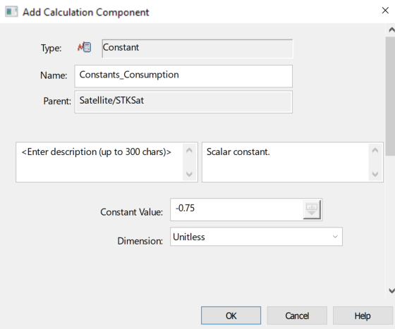
- Enter Constants_Consumption in the Name field.
- Set the Constant Value field to -0.75 and leave the Dimension as Unitless.
- Click .
Constants Consumption scalar calculation component
Defining constant power consumption over the scenario interval
You need to account for how much constant power is being drawn over the course of the scenario. You want to match the time duration of this scalar calculation with your Scenario Interval.
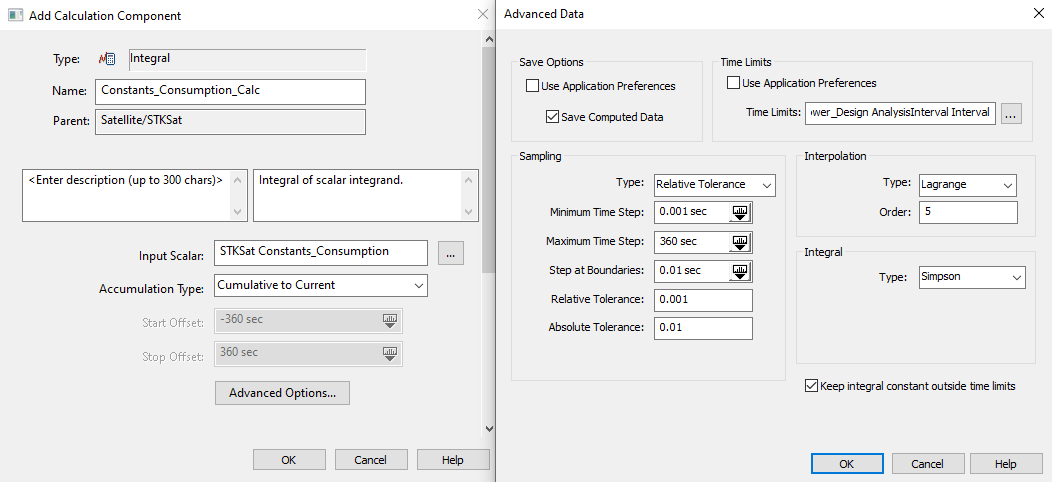
- Click Create new Scalar Calculation ().
- Click Type: when the Add Calculation Component dialog box opens.
- Select Integral () in the Select Component Type list when the Select Component Type dialog box opens.
- Enter Constants_Consumption_Calc in the Name field.
- Set the Input Scalar to the Constants_Consumption ().
- Set the Accumulation Type to Cumulative to Current.
- Set the scenario analysis interval as the time limits for the scalar calculation:
- Click .
- Click the Time Limits ellipsis ().
- Select SolarPowerDesignStarter () in the object tree.
- Select the AnalysisInterval () component in the Components for: SolarPowerDesignStarter list.
- Click three times to create the new Scalar Calculation.
Constant power consumption scalar calculation component
Calculating total power consumption
In this section, the final Scalar Calculation (![]() ) will combine the variable power consumption and the constant power consumption calculations to determine the total power consumption.
) will combine the variable power consumption and the constant power consumption calculations to determine the total power consumption.
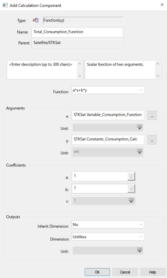
- Select STKSat () in the object tree.
- Click Create new Scalar Calculation ().
- Click Type: when the Add Calculation Component dialog box opens.
- Select Function(x,y) () in the Select Component Type list when the Select Component Type dialog box opens.
- Enter Total_Consumption_Function in the Name field.
- Leave the default Function: a*x+b*y.
- Set Variable_Consumption_Function () as the x reference scalar calculation:
- In the Arguments panel, click the x ellipsis ().
- Select Variable_Consumption_Function () in the Scalar Calculations for: STKSat list.
- Click .
- In the Arguments panel, click the x ellipsis (
- Set Constants_Consumption_Calc () as the y reference scalar calculation:
- In the Arguments panel, click the y ellipsis ().
- Select Constants_Consumption_Calc () in the Scalar Calculations for: STKSat list.
- Click .
- In the Arguments panel, click the y ellipsis (
- Leave all other values their default and click .
Total Consumption scalar calculation
Note: The Total Power Consumption (![]() ) scalar calculation will be used to run a report and exported to Excel for further analysis.
) scalar calculation will be used to run a report and exported to Excel for further analysis.
Generating a Total Power Consumption report
Run a report using the Total Power Consumption (![]() ) scalar calculation and export the results to Excel for further analysis.
) scalar calculation and export the results to Excel for further analysis.
- Right-click on the Total_Consumption_Function () scalar calculation.
- Select Report/Graph... in the shortcut menu.
- Select Total_Consumption_Function_Rate (
 ) in the Select Report Elements list. Leave all other values their default.
 - Click .
- In the Report window, click Save as .csv ().
- Navigate to your desired save location.
- Rename the CSV file to Total Power Consumption Rate.
- Click .
- Close the Report and Analysis Workbench windows.
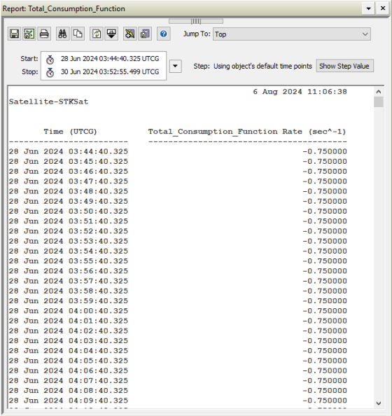
Total Power Consumption Rate report
The Power Generation compared to the Power Consumption is very large. The reason for this is that the battery size and eclipse times of the orbit drive the final selection, instead of the panel efficiency.
Determining the optimal solar panel-battery combination
Use a premade Excel spreadsheet template to condense all of your information together and to run your final analysis. The Excel spreadsheet is set up to adjust the already obtained data to reflect the other efficiencies since the model file uses solar panels with an efficiency of 0.28.
Reviewing the possible solar panel options
The following table lists the three solar panel options for STKSat. The Power Output per Side value represents the total power output of the system of solar panels, not each panel independently.
Solar Panel Options
| Model | Power Output per Side (W) | Efficiency | Cost ($) |
|---|---|---|---|
| Panel System 1 | 2 | 0.28 | 18,000 |
| Panel System 2 | 1.5 | 0.21 | 15,000 |
| Panel System 3 | 1.2 | 0.168 | 12,000 |
Reviewing the possible battery options
The following table lists the three battery options for STKSat.
Battery Options
| Model | Type | Capacity (Wh) | DoD | Cost ($) |
|---|---|---|---|---|
| Battery 1 | Li-ion | 7.5 | 15.0% | 2,000 |
| Battery 2 | Li-ion | 10 | 15.0% | 3,000 |
| Battery 3 | Li-ion | 15 | 15.0% | 4,000 |
Locating the final power analysis spreadsheet template
Open the Final Power Analysis spreadsheet from the lesson files.
- Locate the Excel spreadsheet titled Final Power Analysis Blank.xlsx in the SolarPowerDesignStarter scenario folder.
- Rename the new file Final Power Analysis.
- Open the file in Excel.
Completing your final power analysis spreadsheet
Copy the results from your previously saved power generation and consumption reports into this spreadsheet.
- Open the Total Power Generation report file that you created earlier.
- Copy the entire column of values for Time and Power.
- Paste all the values in cell B12 within the Final Power Analysis spreadsheet to fill Columns B and C.
- Open the Total Power Consumption Rate report file that was created earlier.
- Copy the entire column of values from column B.
- Paste them in cell F12 in the Final Power Analysis spreadsheet. All the values in the spreadsheet should then automatically fill in.
- Observing the solar panel and battery combination costs, select the most cost effective one that satisfies the mission requirements.
In order to paste the values, right-click on your selection and select Values (V) in the Paste Options to keep the column B and C cells colored. In addition, the power values from the Total Power Generation spreadsheet fill the Panel System 1 column since the efficiency of 28% is used within the Discovery model.
Final Results
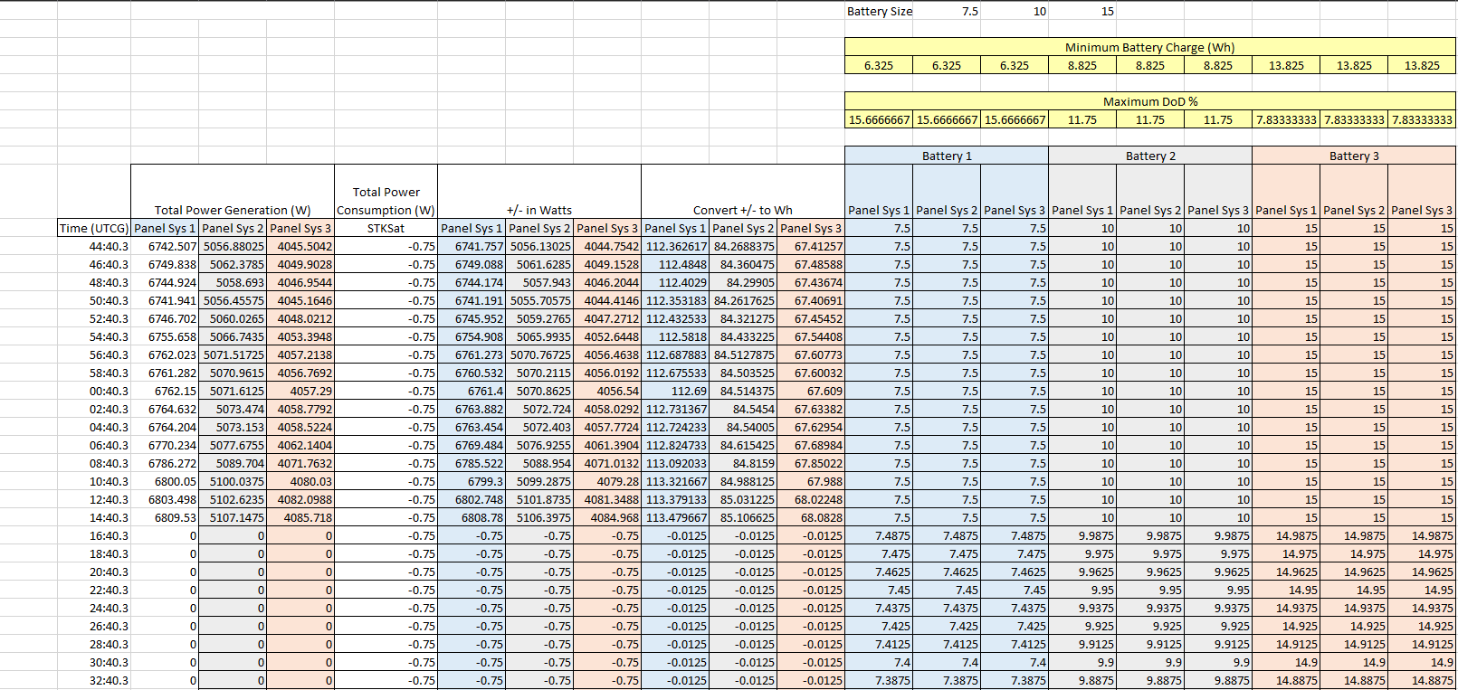
You will find that the best solar panel-battery combination is Battery 1 with Panel System 3. Batteries 2 and 3 were not chosen, as they would surpass their maximum-rated depth of discharge of 15%; according to the Final Power Analysis, the maximum DoD for Battery 1 does not surpass this rated value. After determining that there is one viable battery option, the solar panel system was chosen based on the aspect of cost. The most cost-effective EPS combines Battery 1 with Panel System 3, since that solar panel system has the lowest cost of $14,000.
Updating STKSat's model
You were only modeling STKSat's solar panels in this lesson for the purpose of analysis. For visualization purposes, you may want to use a high-fidelity model that has had textures and additional articulation points applied for added realism.
- Right-click on STKSat () in the Object Browser.
- Select Properties () in the shortcut menu.
- Select the 3D Graphics - Model page.
- Click the Model File ellipsis ().
- Browse to the location of the STKSatModel.glb file when the file dialog box opens.
- Select STKSatModel.glb.
- Click to accept your change and to load the new model.
- Click .
Notice that the untextured model that was produced using the Ansys Discovery software has been replaced with one that looks more realistic.
Updated STKSat model
Clearing accesses
Clean up your scenario by clearing the computed accesses.
- Select the Analysis menu.
- Select Access... ().
- Click Clear All Computed Accesses (
 ).
). - Click to close the Access tool.
Saving your work
Clean up your workspace and close out your scenario to prepare for the next lesson in the Space Mission Analysis and Design series.
- Close all reports and windows except the 2D and 3D Graphics windows.
- Save (
 ) your work.
Summary
You explored the power generation and consumption by subsystems on board a satellite to aid in the design of its EPS. Throughout the process, you created multiple Excel workbooks by saving different reports as CSV files, which allowed you to calculate solar power generation and consumption by the satellite's subsystems. You used the Solar Panel tool to identify the month that would have the least amount of power generated by its solar panels. You also determined when the satellite would be within earth's shadow during that month. You calculated the time of the longest access interval between the satellite and the ground site during those periods of darkness, which would be when the satellite would draw the most power to transmit data while generating the least. You used the Analysis Workbench capability to create multiple scalar calculations to determine the total power consumption by the satellite's subsystems during that time. That information, along with total power generation values from your solar panel analyses, allowed you to find the optimal combination of battery and solar panel system for its EPS that best satisfied the mission requirements.
Space Mission Analysis and Design Part 3: Communications Design
The