STK Premium (Space) or STK Enterprise
You can obtain the necessary licenses for this tutorial by contacting AGI Support at support@agi.com or 1-800-924-7244.
Required product install: The Ansys ModelCenter® model-based systems engineering software and the STK Plugin for ModelCenter are required to complete this tutorial.
ModelCenter installation prerequisites: The ModelCenter software requires the installation of a 64-bit version of Java, a 64-bit implementation of Python 3.x, and the installation of the thrift and six Python packages. See the ModelCenter Installation Prerequisites for more information.
This tutorial was written using version 2026 R1 of the Ansys ModelCenter® model-based systems engineering software.
The results of the tutorial may vary depending on the user settings and data enabled (online operations, terrain server, dynamic Earth data, etc.). It is acceptable to have different results.
Capabilities covered
This lesson covers the following capabilities of the Ansys Systems Tool Kit® (STK®) digital mission engineering software:
- STK Pro
- STK SatPro
- Coverage
- STK Analyzer
Problem statement
Engineers and operators require a quick and easy way to study future satellite constellation designs. You are designing a Walker constellation, which is a group of satellites in circular orbits that have the same period and inclination. Your Walker constellation will employ synthetic-aperture radars (SAR) to create three-dimensional reconstructions of the Earth's land masses. The analysis will require the use of shapefiles, which store data for geographic features. You don't have software developers on your team, so another requirement is a simple trade study tool, which you need to quickly perform "what if" analysis on, collect data from, and subsequently optimize your model.
Solution
Use the STK software's SatPro and Coverage capabilities and the Analyzer capability, which is part of the Ansys ModelCenter® model-based systems engineering software, to determine what your coverage of the Earth's land masses will be over a 24-hour period, considering different variations of altitude on your constellation's satellites.
What you will learn
Upon completion of this tutorial, you will understand how to:
- Create a Walker satellite collection
- Use shapefiles with the Coverage capability
- Analyze a satellite constellation using the ModelCenter software
Creating a new scenario
First, you must create a new STK scenario and then build from there.
- Launch the STK application (
 ).
). - Click
 Create a Scenario in the Welcome to STK dialog box.
 - Enter the following in the New Scenario Wizard:
- Click when you finish.
- Click Save (
 ) when the scenario loads. The STK software creates a folder with the same name as your scenario for you.
 - Verify the scenario name and location in the Save As window.
- Click .
| Option | Value |
|---|---|
| Name | Walker_Analyzer |
| Location | Default |
| Start | Default |
| Stop | Default |
Save (![]() ) often during this lesson!
) often during this lesson!
Disabling streaming terrain
Streaming terrain will not be used in your analysis. You can turn it off for your analysis.
- Right-click on Walker_Analyzer () in the Object Browser.
- Select Properties (
 ).
). - Select the Basic - Terrain page when the Properties Browser opens.
- Clear the Use terrain server for analysis check box in the Terrain Server panel.
- Click to accept your change and to close the Properties Browser.
Creating a Walker satellite constellation
Walker constellations are based on a simple design strategy for distributing the satellites. There are two main Walker constellation variants: Walker-Delta constellations and Walker-Star constellations. The two variants differ in the distribution of the ascending nodes between the planes of the constellation: in a Delta configuration, the ascending nodes of the planes are distributed over a full 360-degree range, while in a Star configuration, the ascending nodes are distributed over a 180-degree span.
Creating a seed satellite
The
- Bring the Insert STK Objects Tool (
 ) to the front.
 - Select Satellite (
 ) in the Insert STK Objects tool.
 - Select the Orbit Wizard (
 ) method.
 - Click .
- Set the following in the Orbit Wizard:
- Look at the Approximate Altitude value of 400 km in the Position panel. This will be discussed later in the tutorial.
- Click .
| Option | Value |
|---|---|
| Type | Repeating Ground Trace |
| Satellite Name | SAR_Sat |
Attaching a Sensor object to your seed satellite
If your seed satellite has sub-objects (child objects) such as sensors, the Walker Tool creates the same sub-objects for each of the child satellites. So, if you want the same grouping of sensors on each of satellites in the constellation, create them on the seed satellite, and the Walker Tool will copy them into the constellation. Insert a
- Insert a Sensor (
 ) object using the Define Properties () method.
 - Select SAR_Sat () in the Select Object dialog box.
- Click .
Using an SAR sensor type
The Sensor objects will model the field of regard of a synthetic aperture radar. A Synthetic Aperture Radar sensor type synthesizes the aperture of a larger antenna than is actually present. It uses SAR pattern definitions designed to model the field of regard of a SAR sensor onto the surface of the earth.
- Select the Basic - Definition page when the Properties Browser opens.
- Open the Sensor Type shortcut menu.
- Select SAR.
- Set the following Elevation Angles:
- Set the following Exclusion Angles:
- Select the Track parent altitude check box.
- Click to accept your changes and to close the Properties Browser.
- Right-click on Sensor1 () in the Object Browser.
- Select Rename in the shortcut menu.
- Rename Sensor1 () SAR_Sens.
| Option | Value |
|---|---|
| Min | 50 deg |
| Max | 90 deg |
| Option | Value |
|---|---|
| Forward | 70 deg |
| Aft | 70 deg |
Enabling this option will force the SAR sensor to track the altitude of its parent object, rather than assuming a constant altitude.
Creating a Walker Satellite collection
You have defined a satellite with the characteristics and orbit you need. Use a Satellite Collection object and the Walker Tool to generate a Walker constellation. A
- Insert a SatelliteCollection (
 ) object using the Walker Tool () method.
 - Click when the Walker Tool opens.
- Select SAR_Sat () in the Select Object dialog box.
- Click to close the Select Object dialog box.
- Set the following values:
- Set the following Container Options:
- Click .
- Click to close the Walker Tool.
- Clear the SAR_Sat () check box in the Object Browser.
| Option | Value |
|---|---|
| Number of Sats per Plane | 2 |
| Number of Planes | 1 |
| Option | Value |
|---|---|
| Select Option | Create Satellite Collection |
| Name | SAR_Sats |
This turns SAR_Sat (![]() ) off visually in both the 2D and 3D graphics windows; it's still available analytically.
) off visually in both the 2D and 3D graphics windows; it's still available analytically.
Using a Satellite Collection reference object
When you use an entry of a satellite collection in your analysis, that entry will inherit the properties of a reference object. By default, the reference object is simply the default satellite object. However, if you choose a default subset reference object, the STK application will associate each member of a subset with that specific satellite in the scenario. Using a specified satellite provides a way to customize settings (attitude, access constraints, etc.) when you use the satellite collection member in an analysis. Moreover, when the reference object contains child objects (sensors, transmitters, receivers, etc.), The STK application also associates these children with the satellite entry. You can then use these children in the analysis tools.
- Open SAR_Sats' () Properties ().
- Select the Basic - Definition page when the Properties Browser opens.
- Click Edit default subset reference object (
 ) for the Default Subset Reference Object.
 - Select SAR_Sat () in the Select Object dialog box.
- Click to close the Select Object dialog box.
- Click .
- Look at the Subsets list. The AllSensors subset is now available.
- Click to accept your changes and to close the Properties Browser.
Using the Coverage capability
The STK software's Coverage capability allows you to analyze the global or regional coverage provided by one or more assets while considering all available accesses. To address area coverage capabilities, Coverage provides you with two STK object classes: Coverage Definition objects and Figure of Merit objects. Before running a Coverage analysis, you must first insert a Coverage Definition object.
Inserting a Coverage Definition object
You want to assess coverage over the Earth's land masses. To do this, you will use a
- Bring the Insert STK Objects Tool () to the front.
- Insert a Coverage Definition (
 ) object using the Insert Default () method.
 - Rename CoverageDefinition1 () Land_Cov.
Defining the Coverage Grid Area of Interest
Coverage analyses are based on the accessibility of assets (objects that provide coverage) and geographical areas. For analysis purposes, the geographical areas of interest are further refined using regions and points defined by the STK application. Points have specific geographical locations and are used in the computation of asset availability. Regions are closed boundaries that contain sets of points. The combination of the geographical area, the regions within that area, and the points within each region is called the
You will use a custom region for your coverage grid. Custom regions are defined using the boundary points of an existing area target or one or more region list files (*.rl) or shapefiles (*.shp). A shapefile is a vector data file format used for geospatial analysis. Shapefiles were developed by ESRI for use with their ArcGIS software but can be
- Open Land_Cov's () Properties ().
- Select the Basic - Grid page when the Properties Browser opens.
- Open the Type drop-down list in the Grid Area of Interest panel.
- Select Custom Regions.
- Select Region File in the drop-down menu below Type.
- Click .
- Browse to the location of the land shapefiles installed with the STK software, typically at C:\Program Files\AGI\STK_ODTK 13\Data\Shapefiles\Land, when the Select Region File dialog box opens.
- Select Land.shp.
- Click .
Specifying the point granularity
When using custom regions, it is important to select adequate point granularity. If a single custom region is smaller than the resolution, the STK application will generate an alternative grid using a finer granularity to ensure at least three samples within the region.
- Enter 4 deg in the Lat/Lon field in the Point Granularity panel.
- Click to accept your changes and to keep the Properties Browser open.
Viewing the Coverage grid
View the Coverage grid in the 2D Graphics window.
- Bring the 2D Graphics window to the front.
- Review the Coverage grid.

Coverage Grid
The Coverage grid points are only on the land masses and include islands. Unlike with Area Target objects, shapefiles support defining polygons with holes. The interior of a polygon is defined to be the area to the right side of the line made by following the points defining the polygon (clockwise). You can therefore create holes in polygons by creating a polygon that overlaps another and has its points defined in the opposite (counterclockwise) order. You can see one such example with the Caspian Sea, which is left out of the coverage definition.
Selecting the coverage assets
Set the satellite sensors as the coverage assets.
- Return to Land_Cov's () Properties ().
- Select the Basic - Assets page.
- Expand (
 ) SAR_Sats () in the Assets list.
 - Select AllSensors (
 ).
). - Click .
- Click .
Turning off Automatically Recompute Accesses
By default, the STK application is set to
- Select the Basic - Advanced page.
- Clear Automatically Recompute Accesses.
- Click to accept your changes and to close the Properties Browser.
Computing accesses
The ultimate goal of coverage is to analyze accesses to an area using assigned assets and applying necessary limitations upon those accesses. Now that your Coverage Definition object is defined, compute accesses by opening the
- Right-click Land_Cov () in the Object Browser.
- Select CoverageDefinition in the shortcut menu.
- Select Compute Accesses in the CoverageDefinition submenu.
- Observe coverage displaying accesses in the 2D Graphics window.
Inserting a Figure of Merit object
The STK software enables you to specify the method by which the quality of coverage is measured using a
- Insert a Figure Of Merit (
 ) object using the Insert Default () method.
 - Select Land_Cov () in the Select Object dialog box.
- Click .
- Rename FigureOfMerit1 () Simple_Cov.
Viewing the quality of coverage
View the coverage in the 3D Graphics window.
- Bring the 3D Graphics window to the front.
- Observe the Simple Coverage assessment over the land masses.
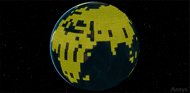
Simple Coverage
Notice there are some holes in your coverage. You can quantitatively gauge just how much with a Percent Satisfied report.
Determining static satisfaction
Generate a Percent Satisfied report to determine the amount of land that is covered by at least one sensor over the 24-hour analysis period. The Static Satisfaction data provider reports the amount of the coverage analysis grid that satisfies satisfaction criteria defined in the figure of merit based on the static definition of the figure of merit. The data provider elements are Percent Satisfied and Area Satisfied.
- Right-click on Simple_Cov () in the Object Browser.
- Select Report & Graph Manager... (
 ) in the shortcut menu.
 - Select the Percent Satisfied (
 ) report in the Installed Styles (
 ) folder in the Styles list when the Report & Graph Manager opens.
 - Click .
- Note the % Satisfied value at the bottom of the report — for example, approximately 90 percent.
You could adjust your satellites and redo your analysis at a variety of altitude until you reached 100 percent coverage, but it would be tedious to repeat the entire scenario time and time again for each altitude that you want to test. Instead, you can use the ModelCenter software to automate your study.
Closing out of the STK application
Before opening the ModelCenter application, clean up and close out of the STK application.
- Close the Percent Satisfied report.
- Close the Report & Graph Manager.
- Save () your scenario.
- Close the STK application.
Creating a new ModelCenter project
The
- Open the ModelCenter (
 ) application.
 - Click in the Welcome to ModelCenter dialog box.
- Click when the What type of model would you like to create? dialog box opens.
- Navigate to your scenario folder (for example, C:\Users\<username>\Documents\STK_ODTK 13\Walker_Analyzer.
- Enter Walker_Analyzer in the File name field.
- Ensure the Save as type is set to the ModelCenter Model (Zip) (*.pxcz).
- Click .
Launching the STK Plugin for ModelCenter
The
- Select favorites (
 ) in the Server Browser at the bottom of the window.
 - Click and drag the STK component (
 ) into the dashed circle underneath "Drop items here to build the model" in the workflow's Analysis View.
 - Select Walker_Analyzer.sc when the Open STK Scenario file dialog box opens.
- Click .
- After a few moments, the STK Analyzer window will open.
The Walker_Analyzer scenario file will open in the STK application in the background.
You can add any of the STK variables as ModelCenter input or output variables through the STK Analyzer window that appears. If you change the value of a variable in your scenario through the STK interface or the ModelCenter Component Tree, you should re-add the variable into ModelCenter or re-run the workflow before running any trade studies with the new value.
Setting up your analysis with Analyzer
Use the STK Analyzer window to configure the input and output variables available for further analysis with the
Selecting the input variables
Use all nine Walker variables as the input variables for your study.
- Select the SAR_Sats () in the STK Variables tree.
- Select the Walker (
 ) property.
 - Move (
 ) Walker () to the Analyzer Variables list.
When you select an object in the STK Variables tree, all possible input variable candidates for that object are listed under the General tab and the Active Constraints tab in the STK Property Variables panel.
Note that the nine Walker variables ( ) are all listed under Inputs in the Analyzer Variables list.
Selecting the output variables
The same data providers that are available in the Report & Graph Manager in the STK application are available in the Data Provider Variables tree.
- Expand (
 ) Land_Cov () in the STK Variables tree.
 - Select Simple_Cov ().
- Expand () the Static Satisfaction (
 ) data provider in the Data Provider Variables tree.
 - Select the Percent Satisfied (
 ) data provider element.
 - Move () Percent Satisfied () into the Analyzer Variables list.
- Click to confirm your selections and to close the STK Analyzer window.
Just like you did with the Figure Of Merit object in your STK scenario, you're looking for changes in percent satisfied at each semi major axis change.
Note that Percent Satisfied ( ) is listed under Outputs in the Analyzer Variables list.
This will also close the STK application, which had been running in the background.
Determining the impact of satellite altitude on coverage
You want to determine the altitude that results in your satellite sensors providing 100-percent coverage of the Earth's land masses. Create a Parametric Study to find this value.
Using the Parametric Study tool
The Parametric Study tool runs a workflow through a sweep of values for some input variable. You can plot the resulting data to view trends.
- Expand () all the elements in the Component Tree.
- Click Parametric Study (
 ) in the Standard toolbar.
 - Click and drag SemiMajorAxis (
 ) from the Component Tree to the Design Variable field when the Parametric Study tool opens.
 - Set the following Design Variable values:
- Click and drag Percent_Satisfied (
 ) from the Component Tree to the Responses field.
 - Click .
| Option | Value |
|---|---|
| starting value | 6900 |
| ending value | 7700 |
| step size | 50 |
Values are in kilometers, the default value for the satellites' semi-major axes. Setting the step size to 50 automatically sets the number of samples to a value of 17, which means your scenario will be analyzed 17 times in 50-kilometer increments between 6,900 and 7,700 kilometers. You want to find the lowest semi-major axis that provides 100-percent satisfaction.
Clicking will open the Data Explorer, which is a tool used by Trade Study tools to display data while they are being collected from your Model. While data are being collected, the Data Explorer displays a progress meter, a halt button, and the data. The Table page of the Data Explorer displays trade study data in a tabular form. It is the default window that is present for all trade studies. Cells are shaded differently depending on the associated variable's state. Input variables are shown with green text, valid values are displayed with black text, invalid values are displayed with gray text, and modified values are displayed with blue text. From the table it is possible to view and edit all values in your trade study and even to add and remove whole runs.
Creating a 2D Line Plot
Once the trade study is complete and all data have been collected, the Data Explorer toolbar becomes active. The Data Explorer stores values for all variables in a workflow and special variables from the trade study. Any variable in the workflow can be plotted against any other variable. Some trade study tools will automatically launch a default plot window when the trade study runs. For other plots, you can create them from the Add View menu. For this study, you will create a 2D Line Plot. A 2D Line Plot displays an X-Y plot for variables in your model.
- Close the 2D Scatter Plot that opened when the trade study finished running.
- Click Add View (
 ) on the Table Page toolbar.
 - Select 2D Line Plot (
 ) in the drop-down menu.
 - Review the 2D Line Plot.
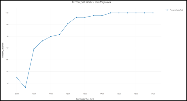
Percent Satisfied versus Semimajor Axis 2D Line Plot
You can see that coverage satisfaction reaches 100 percent at approximately 7,450 kilometers.
Reviewing the Data Explorer table
Look at the Data Explorer table, which provides more specific data about the points on the graph.
- Bring the Table page to the front.
- Select the Chart menu in the Menu Bar.
- Select Show Only Design Variables.
- Scroll until you find the first run where the Percent Satisfied is 100.
- Take a look at the summary of the input and output values.
This will hide all but the variables you are studying with the Parametric Study to make viewing the data easier.

Tabular Data
Your results may vary from those shown above.
You can see that you reach 100-percent satisfaction with a semi-major axis of around 7,450 kilometers for the 24-hour analysis period, which matches what you saw in the 2D Line Plot. You could repeat your Parametric Study, focusing on the range of 7,400 and 7,500 kilometers with smaller step sizes, to find a closer approximation.
Saving your work
Save your work and close out ModelCenter application.
- Close out any open plots, tools, and the Data Explorer window.
- Click when prompted to close your trade study without saving.
- Click Save (
 ) to save your ModelCenter workflow.
 - Close the ModelCenter application.
Summary
This tutorial was an introduction to using the Satellite Collection object and the Walker tool in conjunction with the ModelCenter software. Simple values were used in order to expose you to their functionality. You began the scenario by placing a Satellite object in a repeating ground trace orbit. You attached a Sensor object to the satellite that modeled a synthetic-aperture radar's field of regard. Using the Walker tool to make, you made your Satellite object the seed satellite for a Satellite Collection object to created a simple constellation of two satellites in opposition to each other in one orbital plane. You inserted a Coverage Definition object and assigned a shapefile as your grid area of interest, which covered all the Earth's land masses, and assigned the Sensor objects as the coverage assets. Using a Figure Of Merit object and a Simple Coverage definition, you determined that approximately 90 percent of the Earth's land mass was accessed by the two SAR sensors during a 24-hour analysis period. Using the ModelCenter software's Parametric Study tool, you varied the Satellite object's semi-major axis to study satisfaction percentage at various altitudes.