STK Pro, STK Premium (Air), STK Premium (Space), or STK Enterprise
You can obtain the necessary licenses for this tutorial by contacting AGI Support at support@agi.com or 1-800-924-7244.
This lesson requires STK 12.8 or newer to complete it in its entirety.
The results of the tutorial may vary depending on the user settings and data enabled (online operations, terrain server, dynamic Earth data, etc.). It is acceptable to have different results.
Capabilities covered
This lesson covers the following STK Capabilities:
- STK Pro
- Communications
Problem statement
Engineers and operators require a fast and easy way to analyze digital and analog transponders. They need to up link data from a communications site to a satellite transponder, which will then down link the data to a separate ground site.
Solution
Use STK Pro and the Communications capability to model digital and analog transponders for link budget analysis and mission planning.
What you will learn
Upon completion of this tutorial, you will understand:
- How to model communications involving digital transponders.
- How to model communications involving analog transponders.
- How to generate a Digital Repeater Comm Link report using the Chain object and the Report & Graph Manager.
- How to generate a Bent Pipe Comm Link report using the Chain object and the Report & Graph Manager.
Video guidance
Watch the following video. Then follow the steps below, which incorporate the systems and missions you work on (sample inputs provided).
Using the starter scenario (*.vdf file)
To speed things up and enable you to focus on this lesson's main goal, you will use a partially created scenario. The partially created scenario is saved as a visual data file (VDF) in your STK install.
Retrieving the starter scenario
- Launch the STK (
 ) application.
 - Click
 Open a Scenario in the Welcome to STK dialog box.
 - Go to <Install Dir>\Data\Resources\stktraining\VDFs.
- Select STK_Communications.vdf.
- Click .
Visual data files versus Scenario files
You must make sure that you save your work in the STK application as a scenario file (.sc) and not a visual data file (.vdf) by selecting Save As from the STK File menu. A VDF is a compressed version of an STK scenario, which makes them great for sending your work in the STK application to others. However, you should use a scenario file while working with the STK application on your machine.
If you open a VDF file, the STK application keeps it as a VDF and does not automatically convert it to a scenario file. This means that the STK application does not change the file type of your scenario when you launch your scenario. You need to convert the VDF to a Scenario file using Save As.
Saving a VDF file as a Scenario file
Use Save As from the STK File menu to convert the VDF file that you opened into a scenario file.
- Select Save As... in the File menu.
- Select the STK User folder in the navigation pane.
- Right-click in the file and folder browser.
- Select New > Folder in the shortcut menu.
- Rename New Folder to match the title of the scenario.
- Open the folder you just created.
- Enter the name of the folder into the File name field. This will be the Scenario object's name.
- Open the Save as type drop-down menu.
- Select Scenario Files (*.sc).
- Click .
Analyzing a communications system with digital and analog transponders
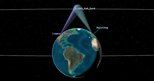
In this scenario, you will analyze communications between a communications ground site located in Southern California, a geosynchronous satellite (GEO), and a communications ground site located in Southern Germany. You will then generate a Digital Repeater Comm Link report and a Bent Pipe Comm Link report to analyze your communications.
Selecting the relevant scenario objects
You will only use a portion of the available objects in the Object Browser in this tutorial, not all of them. There are extra objects because you can use this same scenario to complete other lessons about the STK Communications capability.
- Select the check box for the following objects in the Object Browser:
- Communication_Site (
 )
) - UL_Servo (
 )
) - Raisting (
 )
) - DL_Servo ()
- GEO_Sat_East (
 )
) - Click Save (
 ).
).
Each ground site has a servo system that is tracking the GEO satellite which you can see in the 3D Graphics window.
Save (![]() ) often during this lesson!
) often during this lesson!
Viewing the scene
View the initial scene in the 3D Graphics window for situational awareness.
- Bring the 3D Graphics window to the front.
- Right-click on GEO_Sat_East () in the Object Browser.
- Select Zoom To.
- Use your mouse and zoom out to view the servo motor connections between both ground sites and the satellite.
Servo Motor View
Configuring atmospheric models to your scenario
Configure your scenario to include the ITU-R rain model and the ITU-R atmospheric absorption model. Later in this lesson, you will determine how these conditions affect your communications.
Loading the ITU-R rain model
Use the ITU-R rain model for your analysis.
- Right-click on your Scenario object (
 ) in the Object Browser.
 - Select Properties (
 ).
). - Select the RF - Environment page when the Properties Browser opens.
- Select the Rain, Cloud & Fog tab.
- Select the Use check box in the Rain Model panel.
- Leave the default ITU-R (International Telecommunication Union) model.
- Click to accept the changes and keep the Properties Browser open.
Loading the ITU-R Atmospheric Absorption Model
Use the ITU-R atmospheric absorption model.
- Select the Atmospheric Absorption tab.
- Select the Use check box.
- Leave the default ITU-R model.
- Click to accept your changes and to close the Properties Browser.
Configuring the uplink transmitter
Analyze the communications from the ground site to the satellite's transponders. In order to do that, create an uplink transmitter on a ground site first.
Inserting a Transmitter object
Your parabolic antenna is directional. You can steer the antenna by attaching the Transmitter (![]() ) object to a Sensor (
) object to a Sensor (![]() ) object.
) object.
- Select Transmitter (
 ) in the Insert STK Objects tool.
 - Select the Insert Default () method.
- Click
- Select UL_Servo () in the Select Object dialog box.
- Click .
- Right-click on Transmitter1 () in the Object Browser.
- Select Rename in the shortcut menu.
- Rename Transmitter1 () to Uplink_Tx.
Using a Complex Transmitter model
Use a Complex Transmitter model to analyze the uplink portion of your link analysis. The Complex Transmitter model enables you to select among a variety of analytical and realistic antenna models and to define the characteristics of the selected antenna type.
- Open Uplink_Tx's () Properties ().
- Select the Basic - Definition page.
- Click the Transmitter Model Component Selector (
 ).
). - Select Complex Transmitter Model (
 ) in the Transmitter Models list, once the Select Component dialog box opens.
 - Click to close the Select Component dialog box.
- Enter the following specifications:
- Click to accept your changes and to keep the Properties Browser open.
| Option | Value |
|---|---|
| Frequency | 18 GHz |
| Power | 10 dBW |
| Data Rate | 10 Mb/sec |
Using a parabolic antenna
The communications site uses a parabolic antenna.
- Select the Antenna tab.
- Select the Model Specs sub-tab.
- Click the Antenna Model Component Selector ().
- Select Parabolic () in the Antenna Models list.
- Click to close the Select Component dialog box.
- Enter the following specifications:
- Click to accept your changes and to keep the Properties Browser open.
| Option | Value |
|---|---|
| Design Frequency | 15 GHz |
| Diameter | 3.5 m |
The design frequency doesn't match the uplink frequency. The antenna works in a frequency range of 12 - 18 GHz.
Enabling atmospheric refraction
Atmospheric refraction is the bending of an RF signal as it travels through the atmosphere.
- Select the Basic - Refraction page.
- Select the Use Refraction in Access Computations check box.
- Open the Refraction Model drop-down list.
- Select the ITU-R model.
- Click to accept your changes and to close the Properties Browser.
Configuring a digital transponder on the satellite
In a digital (or regenerative) transponder, the transponder demodulates and then re-modulates the incoming signal before the transponder sends the signal back out. Essentially, the transponder cleans and then re-sends the signal.
![]()
DIGITAL TRANSPONDER SCHEMATIC
The image above shows the path of a signal from a ground station transmitter to a satellite's digital transponder and then from the satellite's digital transponder to a ground site's receiver. The satellite's digital transponder is marked by the dashed box.
The digital transponder receives the signal and cleans out the radio frequency (RF) environmental noise during the demodulation of the incoming signal. Then the digital transponder re-modulates the signal and transmits the “clean” signal to the ground receiver.
The advantage of a digital transponder over an analog transponder is the demodulation/remodulation that cleans up the signal. When the ground site receives a signal from the satellite's digital transponder, the signal has less RF environmental noise because the digital transponder has cleaned out the RF environmental noise that occurred during the uplink and is downlinking a clean signal.
Inserting an uplink satellite receiver
When creating a transponder in the STK application, use a Receiver (![]() ) object and a Transmitter (
) object and a Transmitter (![]() ) object on the same parent object.
) object on the same parent object.
- Insert a Receiver (
 ) object using the Insert Default () method.
 - Select GEO_Sat_East () in the Select Object dialog box.
- Click to close the Select Object dialog box.
- Rename Receiver1 () to Uplink_Rx.
Specifying the receiver model
Use a
- Open Uplink_Rx's () Properties ().
- Select the Basic - Definition page.
- Click the Receiver Model Component Selector ().
- Select Complex Receiver Model () in the Receiver Models list.
- Click to accept your selection and to close the Select Component dialog box.
Adding a parabolic antenna to the receiver
Your satellite receiver will have a parabolic antenna.
- Select the Antenna tab.
- Select the Model Specs sub-tab.
- Click the Antenna Model Component Selector ().
- Select Parabolic () in the Antenna Models list.
- Click to accept your selection and to close the Select Component dialog box.
- Enter 15 GHz in the Design Frequency field.
- Click to accept your changes and to keep the Properties Browser open.
Orienting the antenna using the Az-El orientation method
The Az-El (azimuth-elevation) orientation method specifies the location of the antenna boresight in relation to the azimuth and elevation in the local coordinate frame of the parent object. The receive antenna points in the general direction of the communications site.
- Select the Orientation sub-tab.
- Enter the following specifications:
- Click to accept your changes and to keep the Properties Browser open.
| Option | Value |
|---|---|
| Azimuth | 216.3 deg |
| Elevation | 81.45 deg |
Computing the system noise temperature
Compute system noise temperature.
- Select the System Noise Temperature tab.
- Select the Compute option.
- Select the Compute option in the Antenna Noise panel.
- Select the following options:
- Earth
- Sun
- Atmosphere
- Rain
- Cosmic Background
- Click to accept your changes and to keep the Properties Browser open.
Enabling atmospheric refraction
You can model the effects of atmospheric refraction on the received signal for your anaylsis..
- Select the Basic - Refraction page.
- Select the Use Refraction in Access Computations check box.
- Open the Refraction Model drop-down list.
- Select the ITU-R model.
- Click to accept your changes and to close the Properties Browser.
Inserting a Transmitter object
Add a Transmitter object to the satellite
- Insert a Transmitter () object using the Insert Default () method.
- Select GEO_Sat_East () in the Select Object dialog box.
- Click to close the Select Object dialog box.
- Rename Transmitter2 () to Digital_Downlink_Tx.
Using a Complex Transmitter model
Use a Complex Transmitter model for the downlink portion of your satellite's transponder.
- Open Digital_Downlink_Tx's () Properties ().
- Select the Basic - Definition page.
- Click the Transmitter Model Component Selector ().
- Select Complex Transmitter Model () in the Transmitter Models list.
- Click to accept your selection and to close the Select Component dialog box.
- Select the Model Specs tab.
- Enter the following specifications:
- Click to accept your changes and to keep the Properties Browser open.
| Option | Value |
|---|---|
| Frequency | 16 GHz |
| Power | 5 dBW |
| Data Rate | 5 Mb/sec |
The downlink frequency is lower than the uplink frequency. The path loss of the downlink frequency is smaller and the link needs less transmit power to achieve the required energy per bit to noise density ratio Eb/No and its associated bit error rate (BER).
Adding a parabolic antenna to the transmitter
The satellite transmitter employs a parabolic antenna.
- Select the Antenna tab.
- Select the Model Specs sub-tab.
- Click the Antenna Model Component Selector ().
- Select Parabolic () in the Antenna Models list.
- Click to accept your selection and to close the Select Component dialog box.
- Enter 15 GHz in the Design Frequency field.
- Click to accept your changes and to keep the Properties Browser open.
Using the Az-El orientation method to orient the antenna
The transmit antenna points in the general direction of Raisting.
- Select the Orientation sub-tab.
- Enter the following specifications:
- Click to accept your changes and to keep the Properties Browser open.
| Option | Value |
|---|---|
| Azimuth | 308.5 deg |
| Elevation | 81.44 deg |
Enabling atmospheric refraction
You can model the effects of atmospheric refraction on the transmitted signal.
- Select the Basic - Refraction page.
- Select the Use Refraction in Access Computations check box.
- Open the Refraction Model drop-down list.
- Select the ITU-R model.
- Click to accept your changes and to close the Properties Browser.
Configuring Raisting's downlink receiver
The downlink receiver at Raisting is attached to a servo motor. Use a Complex Receiver model for Raisting's receiver.
Inserting a Receiver object
Add a Receiver object to the servo motor at Raisting.
- Insert a Receiver () object using the Insert Default () method.
- Select DL_Servo () in the Select Object dialog box.
- Click to close the Select Object dialog box.
- Rename Receiver2 () to Downlink_Rx.
Specifying the receiver model
Use a Complex Receiver model.
- Open Downlink_Rx's () Properties ().
- Select the Basic Definition page.
- Click the Receiver Model Component Selector ().
- Select Complex Receiver Model () in the Receiver Models list.
- Click to accept your selection and to close the Select Component dialog box.
Specifying the receiver antenna model
Use the default Gaussian antenna model. The Gaussian antenna model uses an analytical model of a Gaussian beam. The model is like a parabolic antenna within about -6 dB relative to the boresight.
- Select the Antenna tab.
- Select the Model Specs sub-tab.
- Enter the following specifications:
- Click to accept your changes and to keep the Properties Browser open.
| Option | Value |
|---|---|
| Design Frequency | 15 GHz |
| Diameter | 3.5 m |
Computing system noise temperature
Compute system noise temperature.
- Select the System Noise Temperature tab.
- Select the Compute option.
- Select the Compute option in the Antenna Noise panel.
- Select the following options:
- Sun
- Atmosphere
- Rain
- Cosmic Background
- Click to accept your changes and to keep the Properties Browser open.
Enabling atmospheric refraction
You can take into account the effects of atmospheric refraction on the received signal.
- Select the Basic - Refraction page.
- Select the Use Refraction in Access Computations check box.
- Open the Refraction Model drop-down list.
- Select the ITU-R model.
- Click to accept your changes and to close the Properties Browser.
Computing accesses for the digital transponder
To compute access, create a chain object and then generate a Digital Repeater Comm Link report.
Creating the Chain object
A chain is a list of objects in order of access. Assign objects to the chain and define the order in which the objects are accessed.
- Insert a Chain (
 ) object using the Insert Default () method.
 - Rename Chain1 () to Digital_Link.
Defining the start and end objects
Start by choosing the start object and end object in your chain.
- Open Digital_Link's () Properties ().
- Select the Basic - Definition page.
- Click the Start Object ellipsis ().
- Select Uplink_Tx () in the Select Object dialog box.
- Click to close the Select Object dialog box.
- Click the End Object ellipsis ().
- Select Downlink_Rx () in the Select Object dialog box.
- Click to close the Select Object dialog box.
Creating the Chain Object's first connection
After you choose the start and end objects in your chain, you need to build the chain's connections.
- Click in the Connections panel.
- Click the From Object ellipsis ().
- Select Uplink_Tx () in the Select Object dialog box.
- Click to close the Select Object dialog box.
- Click the To Object ellipsis ().
- Select Uplink_Rx () in the Select Object dialog box.
- Click to close the Select Object dialog box.
Creating the Chain Object's second connection
Next, build the second connection in the chain from the uplink receiver to the digital downlink transmitter.
- Click in the Connections panel.
- Click the From Object ellipsis ().
- Select Uplink_Rx () in the Select Object dialog box.
- Click to close the Select Object dialog box.
- Click the To Object ellipsis ().
- Select Digital_Downlink_Tx () in the Select Object dialog box.
- Click to close the Select Object dialog box.
Creating the Chain Object's third connection
Add the final link in the chain to the digital downlink receiver.
- Click in the Connections panel.
- Click the From Object ellipsis ().
- Select Digital_Downlink_Tx () in the Select Object dialog box.
- Click to close the Select Object dialog box.
- Click the To Object ellipsis ().
- Select Downlink_Rx () in the Select Object dialog box.
- Click to close the Select Object dialog box.
- Click to accept your changes and to close the Properties Browser.
Generating a Digital Repeater Comm Link report
Use the Report & Graph Manager to analyze the performance of your communication link using the Digital Repeater Comm Link report.
- Right-click on Digital_Link () in the Object Browser.
- Select Report & Graph Manager... (
 ) in the shortcut menu.
 - Select Digital Repeater Comm Link (
 ) in the Installed Styles list once the Report & Graph Manager opens.
 - Click
- Scroll to the BER Tot . 2 column when the report opens.
- Click Save as quick report (
 ) in the report tool bar.
For each reported access, the first line of the report is the uplink and the second line the downlink. BER Tot . 2 is the composite. You'll see that for several elements of performance, such as BER, while there may be degradation in the uplink or downlink, minimal degradation or increase is noted in the composite link. If technicians at Raisting are basing reception on a BER of 1.000000e-10 or lower, they can use this report to determine when they have good communications during the 24 hour analysis period.
Preparing for the next section
- Close any open reports, properties and the Report & Graph Manager.
- Clear the Digital_Link () check box in the Object Browser.
Configuring an analog transponder on the satellite
In an analog transponder, the transmitted signal is essentially a reflection of the received signal, with the added possibility of frequency translation or power amplification:
![]()
ANALOG TRANSPONDER SCHEMATIC
Analog transponders do not clean up a received signal before transmitting it out again. Whatever RF environmental noise goes into the analog transponder during the uplink is what you get during the re-transmission of the signal plus any RF environmental noise that's accumulated during the downlink.
You can use STK Communications to determine how RF environmental noise will affect your link budget during your analytical period.
Copying the digital downlink transmitter object
Reuse Digital_Downlink_Tx (![]() ) with some modifications to model an analog downlink transponder.
) with some modifications to model an analog downlink transponder.
- Select Digital_Downlink_Tx () in the Object Browser.
- Click Copy (
 ) in the Object Browser toolbar.
 - Select GEO_Sat_East ().
- Click Paste (
 ).
). - Rename Digital_Downlink_Tx1 () to Analog_Downlink_Tx.
Using the complex retransmitter model
The complex retransmitter model allows you to select among a variety of analytical and realistic antenna models and to define the characteristics of the selected antenna type.
- Open Analog_Downlink_Tx's () Properties ().
- Select the Basic - Definition page.
- Click the Transmitter Model Component Selector ().
- Select Complex Re-Transmitter Model () in the Transmitter Models list.
- Click to accept your selection and to close the Select Component dialog box.
- Select the Model Specs tab.
- Enter the following specifications:
- Click to accept your changes and to keep the Properties Browser open.
- Sat. Power or Saturation Output Power is the RF Power output of the transmitter as measured at the input to the antenna when the amplifier is at its saturated state.
- Sat. Flux Density or Saturation Flux Density is the amplifier's saturation point by the input flux density in dBW/m2. This represents the per carrier flux density for systems supporting multiple carriers per transmitter.
| Option | Value |
|---|---|
| Sat. Power | 15 dBW |
| Sat. Flux Density | -120 dBW/m^2 |
Specifying the analog transmitter antenna
Use the default Gaussian antenna model.
- Select the Antenna tab.
- Enter 15 GHz in the Design Frequency field.
- Click to accept your changes and to keep the Properties Browser open.
Using the Az-El orientation method to orient the antenna
The transmit antenna points in the general direction of the Raisting.
- Select the Orientation sub-tab.
- Enter the following specifications:
- Click to accept your changes and to keep the Properties Browser open.
| Option | Value |
|---|---|
| Azimuth | 308.5 deg |
| Elevation | 81.44 deg |
Adjusting the transfer function - frequency coefficient
The input and output characteristics of a retransmitter are controlled by transfer functions for the transmit frequency, the input/output backoff characteristics, and the carrier to intermod ratio. The STK software models the transfer functions as Nth-order polynomials by default.
Frequency coefficients specify the transmitted frequency as a function of the received frequency. They can only be entered in polynomial form. The coefficient order displays in the left column of the table and updates automatically as coefficients are added or removed. Input and output units are in Hz. The default coefficients of -7.0e+08 and 1.0 are used to model a 700 MHz down conversion. Your downlink transmitter is transmitting at 16 GHz so you need to adjust the frequency coefficient.
- Select the Transfer Functions tab.
- Select the Frequency sub-tab.
- Change the Index 0 Coefficient to -2e+09.
- Click to accept your changes and to close the Properties Browser.
Computing accesses for the analog transponder
To compute access, create a chain object and then generate a Bent Pipe Comm Link report.
Inserting a Chain object
Insert a Chain object. You must assign objects to the chain and define the order in which the objects are accessed.
- Insert a Chain () object using the Insert Default () method.
- Rename Chain2 () to Analog_Link.
Defining the start and end objects
Start by choosing the start object and end object in your chain.
- Open Analog_Link's () Properties ().
- Select the Basic - Definition page.
- Click the Start Object ellipsis ().
- Select Uplink_Tx () in the Select Object dialog box.
- Click to close the Select Object dialog box.
- Click the End Object ellipsis ().
- Select Downlink_Rx () in the Select Object dialog box.
- Click to close the Select Object dialog box.
Creating the Chain Object's first connection
After you choose the start and end objects in your chain, you need to build the chain's connections.
- Click in the Connections panel.
- Click the From Object ellipsis ().
- Select Uplink_Tx () in the Select Object dialog box.
- Click to close the Select Object dialog box.
- Click the To Object ellipsis ().
- Select Uplink_Rx () in the Select Object dialog box.
- Click to close the Select Object dialog box.
Creating the Chain Object's second connection
Add the second link in the chain form the uplink receiver to the downlink transmitter.
- Click .
- Click the From Object ellipsis ().
- Select Uplink_Rx () in the Select Object dialog box.
- Click to close the Select Object dialog box.
- Click the To Object ellipsis ().
- Select Analog_Downlink_Tx () in the Select Object dialog box.
- Click to close the Select Object dialog box.
Creating the Chain Object's third connection
Add the final link in the chain from the analog downlink transmitter to the downlink receiver.
- Click .
- Click the From Object ellipsis ().
- Select Analog_Downlink_Tx () in the Select Object dialog box.
- Click to close the Select Object dialog box.
- Click the To Object ellipsis ().
- Select Downlink_Rx () in the Select Object dialog box.
- Click to close the Select Object dialog box.
- Click to accept your changes and to close the Properties Browser.
Generating a Bent Pipe Comm Link report
You are transmitting data from the uplink transmitter to the uplink receiver. The uplink receiver is transferring the data to the downlink transmitter. Then the downlink transmitter is sending the data to the downlink receiver like a bent pipe. The only processing performed is to retransmit the signal. Any signal degradation is passed on to the downlink receiver. Analyze the reception at Raisting using a Bent Pipe Comm Link report.
- Right-click on Analog_Link () in the Object Browser.
- Select Report & Graph Manager... () in the shortcut menu.
- Select the Bent Pipe Comm Link () report in the Installed Styles list once the Report & Graph Manager opens.
- Click
- Leave the Bent Pipe Comm Link report open.
- Open the Quick Report Manager... (
 ) menu in the Data Providers toolbar at the top of the STK application.
 - Select Digital Repeater Comm Link.
- Display the Bent Pipe Comm Link and Digital Repeater Comm Link reports so that you can view them simultaneously on the screen.
The report contains link performance data for the uplink (first line), downlink (second line), and the combined link (third line). Degradation in downlink and composite link performance can readily be perceived. For example, if you look at the first access line Bit Error Rate (BER) is ~ 2.4 x 10‐14 in the uplink, 1 x 10‐30 in the downlink, and BER Tot .2 is ~ 9.5 x 10‐13 in the composite link. If basing your communications on BER, you would use BER Tot .2 to determine when you can receive data.
You can see that the uplink performance for the analog and digital links are similar and that the analog link downlink performance is improved over the digital downlink performance. However, the composite link performance is better for the digital transponder. This is due to, among other things, the fact that the noise in the uplink channel is propagated through the downlink by the analog transponder but not by the digital transponder.
Saving your work
Clean up your workspace and save your scenario.
- Close any open reports, the Access Tool, and properties.
- Save () your work.
Summary
When you are using the STK software for communications analysis, it's not only important to know how to create a link budget between a transmitter and a receiver, but you need to understand how to model transponders.
In this lesson, you learned how to create digital and analog transponders, the difference being the satellite transmitter model used in your analysis. In your analysis, the digital transponder on the satellite used a Complex Transmitter model (but in reality, you could have used Simple or Medium Transmitter models). You used a Chain object and generated a Digital Repeater Comm Link report and saw that link performance may degrade in the downlink but minimal degradation occurred in the composite link. Basically, the signal was reprocessed and cleaned up prior to retransmission.
For the analog link, you used a re-transmitter model for your satellite's transmitter. Next, you generated a Bent Pipe Comm Link report and saw that link performance was good in the downlink but degraded in the composite link due to noise in the uplink channel which was propagated through the downlink.