STK Premium (Space) or STK Enterprise
You can obtain the necessary licenses for this tutorial by contacting AGI Support at support@agi.com or 1-800-924-7244.
The results of the tutorial may vary depending on the user settings and data enabled (online operations, terrain server, dynamic Earth data, etc.). It is acceptable to have different results.
The technical notes for this exercise can be viewed here.
Capabilities covered
This lesson covers the following capabilities of the Ansys Systems Tool Kit® (STK®) digital mission engineering software:
- STK Pro
- Astrogator
Problem statement
Engineers and operators want to transfer a satellite from a low-Earth parking orbit with a radius of 6,700 kilometers to an outer circular orbit with a radius of 42,238 kilometers. While a Hohmann transfer is the most efficient two-burn maneuver to use in this situation, it is also one of the slowest. Among other things, the satellite is required to travel the entire length of the elliptical transfer orbit, including the approach to apoapsis, where its velocity is considerably slower than in the portion of the orbit near periapsis. If it is of great importance to reduce the time of flight (e.g. for a rendezvous or a planetary intercept) a maneuver such as that shown in the illustration in the technical notes for this exercise can be used. This maneuver, known as a fast transfer, is considerably faster than a Hohmann transfer, but it uses more fuel.
Solution
Use the STK/Astrogator® capability to design a fast transfer from a 6,700 kilometer parking orbit to a 42,238 kilometer outer orbit using Mission Control Sequence segments. Then, design a one tangent burn to fast transfer another satellite from a 6,700 kilometer parking orbit to a 14,000 kilometer outer orbit.
What you will learn
Upon completion of this tutorial, you will be able to:
- Design a fast transfer using Target Sequences
- Customize multiple control parameters and equality constraints
- Design a one tangent burn
Video guidance
Watch the following video. Then follow the steps below, which incorporate the systems and missions you work on (sample inputs provided).
Creating a new scenario
First, you must create a new scenario, and then build from there.
- Launch the STK application (
 ).
). - Click
 Create a Scenario when the Welcome to STK dialog box opens.
 - Enter the following in the STK: New Scenario Wizard:
- Click when you finish.
- Click Save (
 ) when the scenario loads. The STK application creates a folder with the same name as your scenario for you.
 - Verify the scenario name and location in the Save As dialog box.
- Click .
| Option | Value |
|---|---|
| Name | Hohmann_Fast_Transfer |
| Start | 1 Aug 2025 16:00:00.000 UTCG |
| Stop | + 3 days |
Save (![]() ) often during this scenario!
) often during this scenario!
Cleaning up your workspace
The Timeline View and the 2D Graphics window aren't needed in this scenario.
- Close (
 ) the 2D Graphics window.
 - Close () the Timeline View.
Inserting a Satellite object
Insert a Satellite object and name it Fast_Transfer.
- Bring the Insert STK Objects tool (
 ) to the front.
 - Select Satellite (
 ) in the Select An Object To Be Inserted list.
 - Select Insert Default () in the Select A Method list.
- Click .
- Right-click on Satellite1 () in the Object Browser.
- Select Rename in the shortcut menu.
- Rename Satellite1 () Fast_Transfer.
Setting the 3D Graphics Pass properties
Choose how you want to display the Satellite object's orbit in the 3D Graphics window on the
- Right-click on Fast_Transfer () in the Object Browser.
- Select Properties (
 ) in the shortcut menu.
 - Select the 3D Graphics - Pass page when the Properties Browser opens.
- Open the Lead Type drop-down list in the Orbit Track panel.
- Select All.
- Click to confirm your changes and to keep the Properties Browser open.
The Lead Type defines the display of the leading portion of a vehicle's track. Selecting All displays the track spanning the entire vehicle ephemeris.
Changing the propagator to Astrogator
The
- Select the Basic - Orbit page.
- Open the Propagator drop-down list.
- Select Astrogator.
Setting up the Mission Control Sequence
The Mission Control Sequence (MCS) is the core of your space mission scenario. The MCS functions as a graphical programming language, in which mission segments dictate how Astrogator calculates the trajectory of the spacecraft based on the general settings that you specify for the MCS itself.
The MCS is defined by selecting and organizing MCS Segments in a manner that produces your desired trajectory. The left side of the MCS is represented schematically by a tree structure, which lists the segments that make up the MCS and depicts their relationships to each other. Above the tree is the MCS toolbar, which contains buttons that perform various MCS and individual segment operations. By default, the MCS contains Initial State and Propagate segments that produce a low Earth orbit. The right side of the window contains the parameters of the segment that is currently selected in the MCS Tree.
Defining the Initial State segment
Use the
- Select Initial State (
 ) in the MCS.
 - Select the Elements tab.
- Open the Coordinate Type drop-down list.
- Select Keplerian.
- Set the following orbital parameters:
- Keep the rest of the default settings.
- Click to confirm your changes and to keep the Properties Browser open.
The Classical coordinate type uses the traditional osculating Keplerian orbital elements to specify the shape and size of an orbit.
| Option | Value |
|---|---|
| Semi-major Axis | 6700 km |
| Inclination | 0 deg |
Setting the fuel tank configuration
Set the maximum fuel mass and the fuel mass of the
- Select the Fuel Tank tab.
- Enter the following values:
- Click to confirm your changes and to keep the Properties Browser open.
| Option | Value |
|---|---|
| Maximum Fuel Mass | 5000 kg |
| Fuel Mass | 5000 kg |
Propagating the parking orbit
Use the Propagate segment to model the movement of the spacecraft along its current trajectory until meeting specified stopping conditions. The segment uses the defined propagator and integrator to propagate the orbital state, adding each point to the ephemeris as it goes.
- Select Propagate (
 ) in the MCS.
 - Click Segment Properties () in the MCS toolbar.
- Enter Parking Orbit in the Name field of the Edit Segment dialog box.
- Click to confirm your change and to close the Edit Segment dialog box.
Setting the stopping condition
- Look in the Stopping Conditions panel.
- Notice that the default stopping condition for Parking Orbit is Duration.
- Enter 7200 sec in the Trip field.
- Click to confirm your changes and to keep the Properties Browser open.
7,200 seconds, or 2 hours, is more than enough time to have the satellite orbit one complete pass.
Using a Target Sequence to place the satellite into a transfer ellipse
In this scenario, use a Target Sequence to calculate the Delta-V required to move the spacecraft from the parking orbit into the transfer orbit and finally the outer orbit. The goal of the Target Sequence will be defined in terms of the radius of apoapsis of the transfer ellipse, twice the radius of the desired final orbit. This is how you create a fast transfer.
Adding a Target Sequence
Add a
- Select Parking Orbit () in the MCS.
- Click Insert Segment After (
 ) in the MCS toolbar.
 - Select Target Sequence (
 ) in the Segment Selection dialog box.
 - Click to confirm your selection and to close the Segment Selection dialog box.
- Right-click on Target Sequence () in the MCS.
- Select Rename in the shortcut menu.
- Rename Target Sequence () Start Transfer.
Inserting an Impulsive Maneuver segment
For an
- Right-click on the Return (
 ) segment that's nested within Start Transfer ().
 - Select Insert Before... in the shortcut menu.
- Select Maneuver (
 ) in the Segment Selection dialog box.
 - Click to confirm your selection and to close the Segment Selection dialog box.
- Notice that the default Maneuver Type is Impulsive.
Changing the segment properties
Change the name of the Maneuver segment.
- Select Maneuver () in the MCS.
- Click Segment Properties () in the MCS toolbar.
- Enter DV1 in the Name field of the Edit Segment dialog box.
- Click to confirm your change and to close the Edit Segment dialog box.
- Click to confirm your change and to keep the Properties Browser open.
Setting the satellite's attitude and variable
The Attitude Control field enables you to select the mode in which the maneuver pointing direction is prescribed. Use the default Attitude Control setting of Along Velocity Vector. The satellite object’s attitude is such that the Delta-V vector aligns with the spacecraft's inertial velocity vector. The inertial reference frame depends on the central body of the satellite object. Either the thruster set or an engine model defines the Delta-V in the body frame.
- Select the Attitude tab.
- Notice that the Attitude Control defaults to Along Velocity Vector.
Selecting the independent variable
A Target Sequence's differential corrector profile uses a differential correction algorithm to achieve a goal value or set of values. The values that the profile targets are called independent variables, or control parameters. The values that define the goal of the profile are called dependent variables, or equality constraints (or results). When the Target Sequence runs, it will change the values of the independent variables to achieve the goal. You can use any element of a nested MCS segment or linked component as an independent variable. Use Delta-V Magnitude. Delta-V Magnitude is the magnitude of the impulse to be added to the spacecraft velocity vector in distance / time.
- Click on the Delta-V Magnitude target (
 ).
). - Click to confirm your changes and to keep the Properties Browser open.
Notice the target now has a check mark (![]() ). Selecting the target makes Delta-V Magnitude an independent variable. This tells Astrogator to determine the Delta-V based on user determined results.
). Selecting the target makes Delta-V Magnitude an independent variable. This tells Astrogator to determine the Delta-V based on user determined results.
Updating mass based on fuel usage
The Engine tab defines the magnitude and the nature of the propulsion. The Engine parameters specified on this tab are used primarily to define the maneuver direction when using a thruster set to seed a finite maneuver and to update the fuel mass. By selecting Update Mass Based on Fuel Usage, Astrogator updates the mass of the spacecraft as fuel is consumed.
- Select the Engine tab.
- Select the Update Mass Based on Fuel Usage check box.
- Click to confirm your changes and to keep the Properties Browser open.
Selecting the results variable
Dependent variables for a differential corrector profile are defined in terms of calculation objects.
- Click at the bottom of the MCS.
- Expand (
 ) the Keplerian Elems (
 ) folder in the Available Components list when the User - Selected Results - DV1 dialog box opens.
 - Select Radius Of Apoapsis (
 ).
). - Click Insert Component (
 ) to move Radius Of Apoapsis () to the selected components list.
 - Click to close the User - Selected Results - DV1 dialog box.
- Click to confirm your changes and to keep the Properties Browser open.
Setting up the differential corrector profile
Selecting run active profiles runs the Mission Control Sequence allowing the active profiles to operate.
- Select Start_Transfer () in the MCS.
- Open the Action drop-down list.
- Select Run active profiles.
Setting the independent variable
Set up the differential corrector profile to change the Delta-V magnitude to achieve a desired radius of apoapsis. Use magnitude as the control parameter (independent variable).
- Select Differential Corrector in the Profiles panel.
- Click Properties... () in the Profiles toolbar.
- Select the Use check box for ImpulsiveMnvr.Pointing.Spherical.Magnitude in the Control Parameters panel when the Differential Corrector dialog box opens.
Setting the dependent variable
Set radius of apoapsis as the equality constraint (result) with a goal of 84,476 kilometers. Astrogator will use radius of apoapsis to determine the required Delta-V.
- Select the Use check box for Radius_Of_Apoapsis in the Equality Constraints (Results) panel.
- Click the Desired Value cell.
- Enter 84476 km in the Desired Value cell.
- Click to confirm your changes and to close the Differential Corrector dialog box.
- Click to confirm your changes and to keep the Properties Browser open.
Inserting a Propagate segment
Insert a new Propagate segment.
- Right-click on the bottommost Return () segment in the MCS.
- Select Insert Before... in the shortcut menu.
- Select Propagate () in the Segment Selection dialog box.
- Click to confirm your selection and to close the Segment Selection dialog box.
Changing the segment properties
Change the name and color of the Propagate segment.
- Select Propagate () in the MCS.
- Click Segment Properties () in the MCS toolbar.
- Enter Transfer Ellipse in the Name field of the Edit Segment dialog box.
- Open the Color drop-down list.
- Select a color that's different from Parking Orbit ().
- Click to confirm your changes and to close the Edit Segment dialog box.
- Click to confirm your changes and to keep the Properties Browser open.
Propagate segments can be viewed in the 3D Graphics window. By changing the color of each Propagate segment (if you have multiple Propagate segments), you can view them visually. You configured the 3D Graphics Pass properties so that the Maneuver segments nested within the Target Sequences won't be visible in the 3D Graphics window when you propagate the satellite.
Inserting an R Magnitude stopping condition
Use the R Magnitude stopping condition to stop on a specified distance from the origin.
- Click New... (
 ) in the Stopping Conditions panel toolbar.
 - Select R Magnitude () in the New Stopping Condition dialog box.
- Click to confirm your selection and to close the New Stopping Condition dialog box.
- Enter 42238 km in the Trip field.
- Select the Duration stopping condition.
- Click Delete (
 ) in the stopping conditions toolbar.
 - Click to confirm your changes and to keep the Properties Browser open.
Using a second Target Sequence to place the satellite into the outer orbit
Here you will use another Target Sequence to calculate the Delta-V required to break out of the transfer orbit midway to apogee and enter the outer circular orbit. The goal will be to circularize the orbit, i.e., change its eccentricity to zero.
Inserting a new Target Sequence
Insert a new Target Sequence after the Transfer Ellipse Propagate segment.
- Select Transfer Ellipse () in the MCS.
- Click Insert Segment After () in the MCS toolbar.
- Select Target Sequence () in the Segment Selection dialog box.
- Click to confirm your selection and to close the Segment Selection dialog box.
- Right-click on Target Sequence () in the MCS.
- Select Rename in the shortcut menu.
- Rename Target Sequence () Finish Transfer.
Inserting an Impulsive Maneuver segment
Insert a new Maneuver segment into your second Target Sequence.
- Right-click on the Return () segment that's nested within Finish Transfer ().
- Select Insert Before... in the shortcut menu.
- Select Maneuver () in the Segment Selection dialog box.
- Click to confirm your selection and to close the Segment Selection dialog box.
Changing the segment properties
Change the name of the Maneuver segment.
- Right-click on Maneuver () in the MCS.
- Select Rename in the shortcut menu.
- Rename Maneuver () DV2.
- Click to confirm your change and to keep the Properties Browser open.
Setting the satellite's attitude
The Attitude Control field enables you to select the mode in which the maneuver pointing direction is prescribed. Using thrust vector, you specify the Delta-V vector in some reference frame using either Cartesian or spherical components. Astrogator then computes the attitude so that the total thrust vector in the body frame, as specified by the thruster set or engine model, aligns with this vector in the reference axes.
- Select the Attitude tab.
- Open the Attitude Control drop-down list.
- Select Thrust Vector.
Selecting the independent variables
Using Thrust Vector, you will instruct Astrogator to move the satellite in both the X and Z directions.
- Select the X (Velocity) target ().
- Select the Z (Co-Normal) target ().
Updating mass based on fuel usage
Set DV2 to update the satellite's mass based on its fuel usage.
- Select the Engine tab.
- Select the Update Mass Based on Fuel Usage check box.
- Click to confirm your changes and to keep the Properties Browser open.
Selecting the result variables
Select Eccentricity and Flight Path Angle as the calculation components for the Results of the DV2 maneuver.
- Click at the bottom of the MCS.
- Expand () the Keplerian Elems () folder in the Available Components list when the User - Selected Results - DV2 dialog box opens.
- Select Eccentricity ().
- Click Insert Component () to move Eccentricity () to the selected components list.
- Expand () the Spherical Elems () folder in the Available Components list.
- Select Flight Path Angle ().
- Click Insert Component () to move Flight Path Angle () to the selected components list.
- Click to close the User - Selected Results - DV2 dialog box.
- Click to confirm your changes and to keep the Properties Browser open.
Setting up the differential corrector profile
Set up the differential corrector profile to change the X (Velocity) and Z (Co-Normal) to achieve the desired eccentricity and Flight Path Angle.
- Select Finish_Transfer () in the MCS.
- Open the Action drop-down list.
- Select Run active profiles.
Setting the independent variables
Set up the differential corrector profile to use X (Velocity) and Z (Co-Normal) as the control parameters (independent variables).
- Select Differential Corrector in the Profiles panel.
- Click Properties... () in the Profiles toolbar.
- Select the Use check box for ImpulsiveMnvr.Pointing.Cartesian.X in the Control Parameters panel when the Differential Corrector dialog box opens.
- Enter 0.3 km/sec in the Max. Step field.
- Select the Use check box for ImpulsiveMnvr.Pointing.Cartesian.Z.
- Enter 0.3 km/sec in the Max. Step field.
Max Step is the maximum increment to the value of the parameter in a step.
Setting the dependent variables
Leave the Desired Values for Eccentricity and Flight Path Angle at their default values of zero (0).
- Select the Use check box for Eccentricity in the Equality Constraints (Results) panel.
- Select the Use check box for Flight_Path_Angle.
Setting the convergence criteria
Use the Convergence tab to specify convergence criteria and related parameters for the profile. Maximum Iterations define the maximum number of evaluations that the profile will execute. If the profile does not reach the Desired Value, it will stop after the last iteration. The iteration count includes steps taken while searching for bounds as well as bisection iterations.
- Select the Convergence tab.
- Enter 100 in the Maximum Iterations field.
- Click to confirm your changes and to close the Differential Corrector dialog box.
- Click to confirm your changes and to keep the Properties Browser open.
Inserting a Propagate segment
Insert a new Propagate segment.
- Right-click on the bottommost Return () segment in the MCS.
- Select Insert Before... in the shortcut menu.
- Select Propagate () in the Segment Selection dialog box.
- Click to confirm your selection and to close the Segment Selection dialog box.
Changing the segment properties
Change the name and color of the Propagate segment.
- Select Propagate () in the MCS.
- Click Segment Properties () in the MCS toolbar.
- Enter Outer Orbit in the Name field of the Edit Segment dialog box.
- Open the Color drop-down list.
- Select a color that's different from the other Propagate () segments.
- Click to confirm your changes and to close the Edit Segment dialog box.
Setting the duration stopping condition
Use the duration stopping condition.
- Enter 3 day in the Trip Field in the Stopping Conditions panel.
- Click to confirm your changes and to keep the Properties Browser open.
The MCS tree should appear as follows when you are finished. Your colors and names can be different. What's important here are the segments and sequences in the proper locations along with their settings and results.
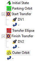
final MCS view
Running the entire Mission Control Sequence
To calculate the trajectory of the spacecraft you must run the Mission Control Sequence. Astrogator will proceed through the MCS and run each segment, generating an ephemeris for the spacecraft. As it runs the MCS, Astrogator carries the trajectory and state of the spacecraft determined so far from one segment to the next.
- Click Run Entire Mission Control Sequence (
 ) in the MCS toolbar.
 - Click Clear Graphics (
 ) in the MCS toolbar.
 - You can view the data in the Targeting Status windows.
- Close the Targeting Status windows when finished.
Viewing the orbit in the 3D Graphics window
You can view the orbit in the 3D Graphics window.
- Bring the 3D Graphics window to the front.
- Use your mouse to obtain a good view of Fast_Transfer as it transfers from a low Earth orbit to the outer orbit.
![]()
fast transfer
When the process is finished, the 3D Graphics window should show a sharp turn from the transfer trajectory into the final orbit, similar to that shown in the illustration. Because of the change in direction, it was necessary to select two components of the second Delta-V as independent variables.
Viewing changes to X (Velocity) and Z (Co-Normal)
You can view the changes to the X (Velocity) and Z (Co-Normal) values in Fast_Transfer's properties.
- Bring Fast_Transfer's () Properties () back to the front.
- Select Finish Transfer () in the MCS.
- Click in the Profiles and Corrections panel.
- Select DV2 () in the MCS.
- Select the Attitude tab.
- Look at the X (Velocity), Z (Co-Normal), and Magnitude values.
- Click to close the Properties Browser.
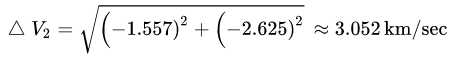
Why are the X (Velocity) and Z (Co-Normal) values negative in DV2? Because you are transferring into a lower-energy orbit and slowing down. You can use these values to compute the value magnitude of Delta-V2. They yield a result that is very close to that reached via the Law of Cosines:
As the
Creating a Maneuver Summary report
Now that you have modeled the satellite's orbit and visualized its behavior, examine the results in a Maneuver Summary report to get an overview about the engine's performance.
- Right-click on Fast_Transfer () in the Object Browser.
- Select Report & Graph Manager... (
 ) in the shortcut menu.
 - Select the Maneuver Summary (
 ) report in the Installed Styles () folder in the Styles panel.
 - Click .
- Scroll through the Maneuver Summary report.
- Close the report and the Report & Graph Manager when you are finished viewing the data.
In defining the Initial State, you set Fuel Mass to 5,000 kilograms. In setting up the two impulsive maneuvers, you opted to have mass decremented on the basis of fuel usage. You can compare how much fuel was required to place your satellite into the outer orbit between this scenario and in the
![]()
Hohmann transfer fuel used
![]()
Fast transfer fuel used
Fast transfer using a one tangent burn strategy
A one tangent burn strategy requires a bigger Delta-V from the initial position, in such a way as to travel the transfer orbit in a shorter amount of time. The angular displacement of the transfer orbit is less than 180 degrees, and a non-tangent burn is executed at the point of intersection of the transfer orbit and the desired final orbit where the intersection angle is equal to the flight path angle of the transfer orbit. Because of this, a precise calculation of the satellite's true anomaly at the intended R Magnitude value is needed prior to executing the final, non-tangent burn.
Similar to the fast transfer you just performed, you want to change the semi-major axis from 6,700 to 14,000 kilometers while maintaining the same inclination and eccentricity for a circular orbit. This time, you will use a Target Sequence to target the true anomaly at a specific, well-defined angular displacement value for your initial tangent burn.
Inserting a Satellite object
Insert a Satellite object and name it OneTangent.
- Insert a Satellite () object using the Insert Default () method.
- Rename Satellite2 () OneTangent.
- Clear Fast_Transfer's () check box in the Object Browser.
Setting the 3D Graphics Pass properties
Set the Lead Type to All to display the orbit track spanning the entire vehicle ephemeris.
- Open OneTangent's () Properties ().
- Select the 3D Graphics - Pass page when the Properties Browser opens.
- Open the Lead Type drop-down list in the Orbit Track panel.
- Select All.
- Click to confirm your changes and to keep the Properties Browser open.
Changing the propagator to Astrogator
Set OneTangent to use Astrogator as its propagator.
- Select the Basic - Orbit page.
- Open the Propagator drop-down list.
- Select Astrogator.
Defining the Initial State segment
Use the Initial State segment to define the initial conditions of your MCS.
- Select Initial State () in the MCS.
- Select the Elements tab.
- Open the Coordinate Type drop-down list.
- Select Keplerian.
- Set the following orbital parameters:
- Keep the rest of the default settings.
- Click to confirm your changes and to keep the Properties Browser open.
| Option | Value |
|---|---|
| Semi-major Axis | 6700 km |
| Inclination | 0 deg |
Setting the Fuel Tank configuration
Set the maximum fuel mass and the fuel mass.
- Select the Fuel Tank tab.
- Enter the following values:
- Click to confirm your changes and to keep the Properties Browser open.
| Option | Value |
|---|---|
| Maximum Fuel Mass | 5000 kg |
| Fuel Mass | 5000 kg |
Setting the Propagate segment's properties
Rename the default Propagate segment.
- Select Propagate () in the MCS.
- Click Segment Properties () in the MCS toolbar.
- Enter Coast in the Name field of the Edit Segment dialog box.
- Click to confirm your change and to close the Edit Segment dialog box.
Setting the stopping condition
Use the duration stopping condition.
- Enter 1000 sec in the Trip field in the Stopping Conditions panel.
- Click to confirm your changes and to keep the Properties Browser open.
Adding a Target Sequence
The first burn is tangential. Add a Target Sequence to calculate the burn's characteristics.
- Select Coast () in the MCS.
- Click Insert Segment After () in the MCS toolbar.
- Select Target Sequence () in the Segment Selection dialog box.
- Click to confirm your selection and to close the Segment Selection dialog box.
- Right-click on Target Sequence () in the MCS.
- Select Rename in the shortcut menu.
- Rename Target Sequence () Transfer.
- Click to confirm your changes and to keep the Properties Browser open.
Inserting an Impulsive Maneuver segment
Insert a new Maneuver segment into the Transfer Target Sequence.
- Right-click on the Return () segment that's nested within Transfer ().
- Select Insert Before... in the shortcut menu.
- Select Maneuver () in the Segment Selection dialog box.
- Click to confirm your selection and to close the Segment Selection dialog box.
Changing the segment properties
Change the name of the Maneuver segment.
- Select Maneuver () in the MCS.
- Click Segment Properties () in the MCS toolbar.
- Enter Tangent Burn in the Name field of the Edit Segment dialog box.
- Click to confirm your change and to close the Edit Segment dialog box.
- Click to confirm your changes and to keep the Properties Browser open.
Selecting the independent variable
You can set an initial guess of 2 km/sec to help the Differential Corrector in getting the correct result.
- Select the Attitude tab.
- Enter 2 km/sec in the Delta-V Magnitude field.
- Select the Delta-V Magnitude target () to make it an independent variable.
- Click to confirm your changes and to keep the Properties Browser open.
Updating mass based on fuel usage
Set Tangent Burn to update the satellite's mass based on its fuel usage.
- Select the Engine tab.
- Select the Update Mass Based on Fuel Usage check box.
- Click to confirm your changes and to keep the Properties Browser open.
Inserting a Propagate segment
Add a Propagate segment nesting it inside the Transfer Target Sequence.
- Select TangentBurn () in the MCS.
- Click Insert Segment After () in the MCS toolbar.
- Select Propagate () in the Segment Selection dialog box.
- Click to confirm your selection and to close the Segment Selection dialog box.
- Click to confirm your changes and to keep the Properties Browser open.
Setting the Propagate segment's properties
Change the name and color of the Propagate segment.
- Select Propagate () in the MCS.
- Click Segment Properties () in the MCS toolbar.
- Enter Prop to RMagnitude in the Name field of the Edit Segment dialog box.
- Open the Color drop-down list.
- Select a color that different from Coast ().
- Click to confirm your change and to close the Edit Segment dialog box.
- Click to confirm your changes and to keep the Properties Browser open.
Setting the stopping condition
Insert an R Magnitude stopping condition.
- Click New... () in the Stopping Conditions panel toolbar.
- Select R Magnitude () in the New Stopping Condition dialog box.
- Click to confirm your selection and to close the New Stopping Condition dialog box.
- Enter 14000 km in the Trip field.
- Select the Duration stopping condition.
- Click Delete () in the stopping conditions toolbar.
Selecting the result variables
Select the calculation objects you will use for the differential corrector profile.
- Click at the bottom of the MCS.
- Expand () the Math () folder in the Available Components list when the User - Selected Results - Prop to RMagnitude dialog box opens.
- Select Difference ().
- Click Insert Component () to move Difference () to the selected components list.
- Double-click on CalcObject in the Component Details list.
- Expand () the Keplerian Elems () folder in the Component Selection dialog box.
- Select True Anomaly ().
- Click to confirm your selection and to close the Component Selection dialog box.
- Click to close the User - Selected Results - Prop to RMagnitude dialog box.
- Click to confirm your changes and to keep the Properties Browser open.
By using the true anomaly as result, you will force the transfer orbit to have a well-defined angular displacement (less than 180 degrees for a one tangent burn) when the orbit arrives at the intended R Magnitude value (14,000 kilometers in this case). You’ll set this parameter to be 140 degrees in the Differential Corrector.
Setting up the differential corrector profile
Set up the differential corrector profile to change the Delta-V Magnitude to achieve the desired result.
- Select Transfer () in the MCS.
- Open the Action drop-down list.
- Select Run active profiles.
Setting the independent variable
Use the impulsive maneuver's spherical magnitude as the control parameter (independent variable).
- Click Properties... () in the Profiles toolbar.
- Select the Use check box for ImpulsiveMnvr.Pointing.Spherical.Magnitude in the Control Parameters panel when the Differential Corrector dialog box opens.
Setting the dependent variable
Use the difference in the true anomaly as an equality constraint (result) with a goal of 140 deg.
- Select the Use check box for Difference in the Equality Constraints (Results) panel.
- Enter 140 deg in the Desired Value cell.
- Click to confirm your selections and to close the Differential Corrector dialog box.
- Click to confirm your changes and to keep the Properties Browser open.
Adding a second Target Sequence
The second burn is non-tangential, so you need to set two control parameters.
- Right-click on the bottommost Return () segment in the MCS.
- Select Insert Before... in the shortcut menu.
- Select Target Sequence () in the Segment Selection dialog box.
- Click to confirm your selection and to close the Segment Selection dialog box.
- Right-click on Target Sequence () in the MCS.
- Select Rename in the shortcut menu.
- Rename Target Sequence () Circularize.
- Click to confirm your changes and to keep the Properties Browser open.
Inserting an Impulsive Maneuver segment
Add a non-tangent burn Maneuver segment to circularize the orbit.
- Right-click on the Return () segment that's nested within Circularize ().
- Select Insert Before... in the shortcut menu.
- Select Maneuver () in the Segment Selection dialog box.
- Click to confirm your selection and to close the Segment Selection dialog box.
Changing the segment properties
Change the name of the Maneuver segment.
- Select Maneuver () in the MCS.
- Click Segment Properties () in the MCS toolbar.
- Enter Non Tangent Burn in the Name field of the Edit Segment dialog box.
- Click to confirm your change and to close the Edit Segment dialog box.
- Click to confirm your changes and to keep the Properties Browser open.
Setting the satellite's attitude
Set the Maneuver segment's attitude control mode to thrust vector.
- Select the Attitude tab.
- Open the Attitude Control drop-down list.
- Select Thrust Vector.
Selecting the independent variables
Instruct Astrogator to move the satellite in both the X and Z directions.
- Select the X (Velocity) target ().
- Select the Z (Co-Normal) target ().
Updating mass based on fuel usage
Set Non Tangent Burn to update the satellite's mass based on its fuel usage.
- Select the Engine tab.
- Select the Update Mass Based on Fuel Usage check box.
- Click to confirm your changes and to keep the Properties Browser open.
Selecting the results variable
Select Eccentricity as the calculation component for the Results of the Non Tangent Burn maneuver.
- Click at the bottom of the MCS.
- Expand () the Keplerian () folder in the Available Components list when the User - Selected Results - Non Tangent Burn dialog box opens.
- Select Eccentricity ().
- Click Insert Component () to move Eccentricity () to the selected components list.
- Select Semimajor Axis ().
- Click Insert Component () to move Eccentricity () to the selected components list.
- Click to confirm your selections and to close the User - Selected Results - Non Tangent Burn dialog box.
Setting up the differential corrector profile
Set up the differential corrector profile to change X (Velocity) and Z (Co-Normal) to achieve the desired semimajor axis and eccentricity.
- Select Circularize () in the MCS.
- Open the Action drop-down list.
- Select Run active profiles.
Setting the independent variables
Set up the differential corrector profile to use X (Velocity) and Z (Co-Normal) as the control parameters (independent variables).
- Click Properties... () in the Profiles toolbar.
- Select the Use check box for ImpulsiveMnvr.Pointing.Cartesian.X in the Control Parameters panel when the Differential Corrector dialog box opens.
- Select the Use check box for ImpulsiveMnvr.Pointing.Cartesian.Z.
Setting the dependent variables
Use the eccentricity and semi-major axis as the equality constraints (Results) to determine the required Delta-V for the non-tangent burn.
- Select the Use check box for Eccentricity in the Equality Constraints (Results) panel.
- Enter 0.01 in the Tolerance field.
- Select the Use check box for Semimajor_Axis.
- Enter 14000 km in the Desired Value cell.
- Click to confirm your selections and to close the Differential Corrector dialog box.
- Click to confirm your changes and to keep the Properties Browser open.
![]()
Differential corrector properties
Inserting a Propagate segment
Insert a new Propagate segment.
- Right-click on the bottommost Return () segment in the MCS.
- Select Insert Before... in the shortcut menu.
- Select Propagate () in the Segment Selection dialog box.
- Click to confirm your selection and to close the Segment Selection dialog box.
Changing the segment properties
Change the name and color of the Propagate segment.
- Select Propagate () in the MCS.
- Click Segment Properties () in the MCS toolbar.
- Enter Final Orbit in the Name field of the Edit Segment dialog box.
- Open the Color drop-down list.
- Select a color that's different from the other Propagate () segments.
- Click to confirm your changes and to close the Edit Segment dialog box.
- Click to confirm your changes and to keep the Properties Browser open.
Setting the duration stopping condition
Use a duration stopping condition for the Final Orbit Propagate segment.
- Insert 3 day in the Trip Field in the Stopping Conditions panel.
- Click to confirm your changes and to keep the Properties Browser open.
The MCS tree should appear as follows when you are finished:
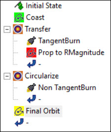
one tangent MCS
Running the entire Mission Control Sequence
Run the entire Mission Control Sequence to propagate the one tangent satellite's orbit.
- Click Run Entire Mission Control Sequence () in the MCS toolbar.
- You can view the data in the Targeting Status windows.
- Close the Targeting Status windows when finished.
- Click Clear Graphics () in the MCS toolbar.
- Click to close the Properties Browser.
Viewing the orbit in the 3D Graphics window
You can view the orbit in the 3D Graphics window.
- Bring the 3D Graphics window to the front.
- Use your mouse to obtain a good view of OneTangent as it transfers from a low Earth orbit to the outer orbit.

one tangent orbit
Creating a Maneuver Summary report
Examine the results with a Maneuver Summary report.
- Right-click on OneTangent () in the Object Browser.
- Select Report & Graph Manager... () in the shortcut menu.
- Select the Maneuver Summary () report in the My Favorites () folder in the Styles panel.
- Click .
- Scroll through the Maneuver Summary report.
- Close the report and the Report & Graph Manager when you are finished viewing the data.
Saving your work
Clean up your workspace and save your work.
- Close any open reports, properties and tools.
- Save () your work.
Summary
Using Astrogator, you transferred a satellite from a low-Earth parking orbit with a radius of 6,700 kilometers to an outer circular orbit with a radius of 42,238 kilometers using a Hohmann transfer. By instructing Astrogator to use a radius of apoapsis out to 84,476 kilometers you stopped the maneuver at 42,238 kilometers using a Propagate segment. In the end, you burnt more fuel to get to the outer orbit, but you got there faster. Using a one tangent burn strategy, you required a large Delta-V in order to travel to a transfer orbit in a shorter amount of time. The altitude of this orbit was 14,000 kilometers. Due to the large Delta-V, a large amount of fuel was required to place the satellite in the final orbit.