Prediction Profiler Page

The Prediction Profiler allows you to visualize and interactively investigate your design space. It allows you to efficiently predict the values of your output variables for any combination of your input variables, visualize slices of the resulting n-dimensional design space (including the effects of constraints), and manually explore and search the design space for good designs.

This tool can be used as a "manual optimizer" to locate good designs or it can be used to find good starting points for a more formal optimization algorithm. It may also be used as a post-processor to visualize the results generated by an optimization algorithm.

To use the Prediction Profiler, utilize the Design of Experiments (DOE) tool or one of the other Trade Study tools to populate the Data Explorer. For best results, it is recommended that the DOE tool be used in conjunction with a "space filling" experimental design such as a Latin-Hypercube design. As a rough guide, generate a design with at least n(n+1)/2 points, where n is the number of design parameters.

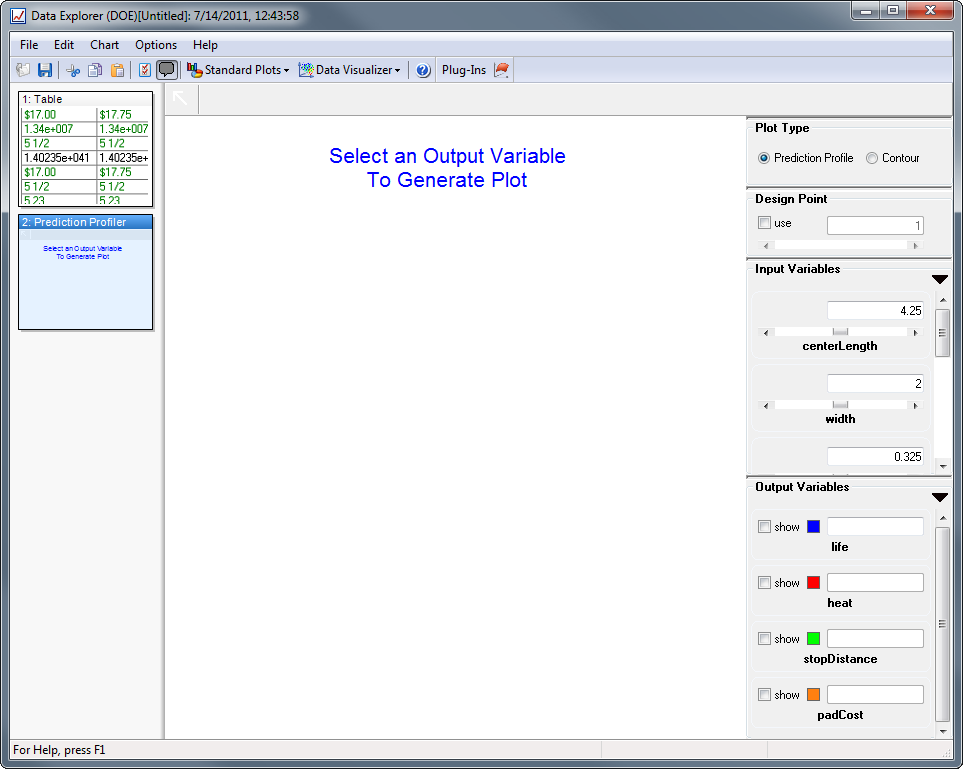
Click the Standard Plots button and select Prediction Profiler from the drop-down menu. When the Prediction Profiler is first displayed, the right-hand control panel will be populated with your input and output variables. The input variables are shown in the top portion of the panel, and the output variables in the bottom portion of the panel.

Analyze Data

Click the checkbox labeled show next to one of your output variables to generate the prediction profiler plots. The first time that an output variable is selected, your data (in the Data Explorer) will be analyzed and a mathematical approximation will be created that will allow you to predict the value of your output variable for different combinations of the input variables. The length of this analysis will depend on the number of input variables, the amount of data that needs to be analyzed, and the nature of the design space. For large problems, this analysis can take several minutes (or more). The analysis can be canceled at any time by pressing the Cancel button. Note that once you have analyzed a given output variable, you may turn it "on" and "off" by clicking on the show checkbox without incurring any additional computational expense.

Click show next to each output variable that you want to analyze.

After the analysis for each selected output variable is complete, you can predict its value for any combination of your input variables -- as long as each input variable is between the upper and lower bounds that you specified when running the DOE tool.

Change the value of an input variable by either (1) typing in a new value in the textbox above the variable name or (2) dragging the slider above the variable name.

When you change the values of the input variables, the predicted output variable values are automatically updated to match.

Your design space can be visualized using either the Profile view or the Contour view. By default, the Profile view is shown.

Profile View

In the Profile view, a series of line plots show the relationship between each of the input variables (on the horizontal axis) and each of the output variables (on the vertical axis) at a particular point in the design space. The black diamonds on each plot correspond to the current values of the input variables (the current design point).

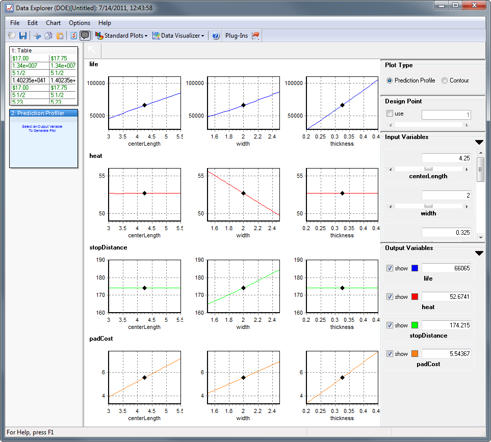
When the input variable values are modified, either by typing new values in the text boxes or dragging the slider bars, the profile plots are updated in real time. You can also change the values of the input variables by clicking anywhere on the profile plots.

By changing the values of the input variables and watching the resulting changes in the output variables, you can explore the design space to find good designs or simply to gain a better feel for the relationships between your variables.

In the above figure it can be seen that, given the current design point, the best way to reduce the stopDistance output variable is to reduce the width input variable, but this will increase the heat. Reducing any of the input variables will decrease the padCost output variable, but will also decrease the life. The centerLength and thickness input variables are predicted to have little to no effect on either the stopDistance or the heat output variables.

The colors used to plot each of the output variables can be changed in the Basic Settings dialog. The Basic Settings dialog can be opened either by double-clicking on the page's thumbnail in the left pane of the Data Explorer or by selecting the Basic Settings option from the Chart menu.

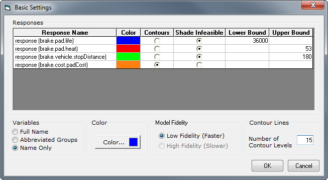
The Basic Settings dialog can also be used to specify upper and lower bounds for one or more of your output variables. If you do this, the portions of your design space that do not satisfy your constraint(s) (regions where output values that are less than your lower bound or greater than your upper bound) will be cross-hatched.

For example, if (in the previous figure) you want the stopDistance to be at less than 180, the heat to be less than 53, and the life to be greater than 36000 you can shade those regions of the design space that don't meet these constraints.

In the Basic Settings dialog, click the button labeled "Shade Infeasible" next to the output variables for which you want to specify lower and/or upper bounds, then enter a value in the "Lower Bound" and/or "Upper Bound" text boxes.

The Profile plots will now be updated to show the feasible (no cross-hatching) and infeasible (cross-hatched) regions of your design space. You can now vary the values of your input variables to determine graphically whether or not your constraints can be met.

Contour View

The Contour view provides an alternate way to view your design space. In the Contour view, you may select any two of your input variables (one for the x-axis and one for the y-axis) and see contours of one or more of your output variables. As with the Profile view, the design space can be explored and investigated in real time.

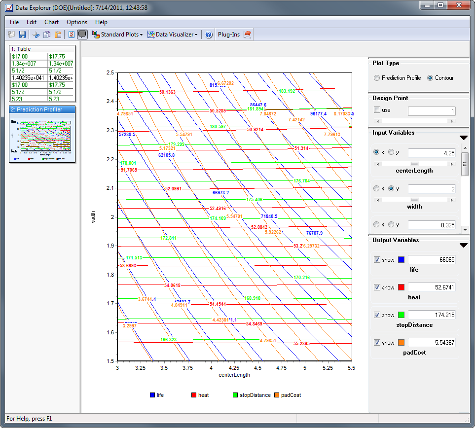
To switch to the Contour View, select the button labeled "Contour" at the top of the right-hand control panel. You may switch back to the Profile view by selecting the button labeled "Prediction Profile".

The black diamond indicates the design point defined by the current values of the input variables. As with the Profile plots, you can change the values of the input variables (and thus the location of the black diamond) by clicking anywhere on the plot.

Specify the input variable to be plotted on the x-axis by clicking the button labeled "x" next to the variable. Likewise, click the button labeled "y" next to an input variable to plot it on the y-axis.

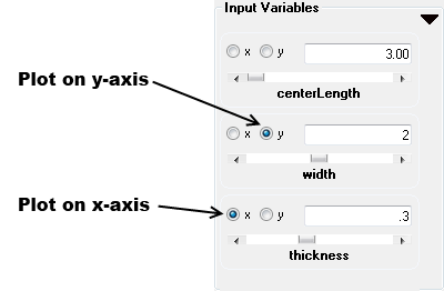
The number of contours shown for the output variables can be modified via the Basic Settings dialog.

If upper and/or lower bounds are specified via the Basic Settings dialog (see above), then the infeasible portions of the design space will be cross-hatched.

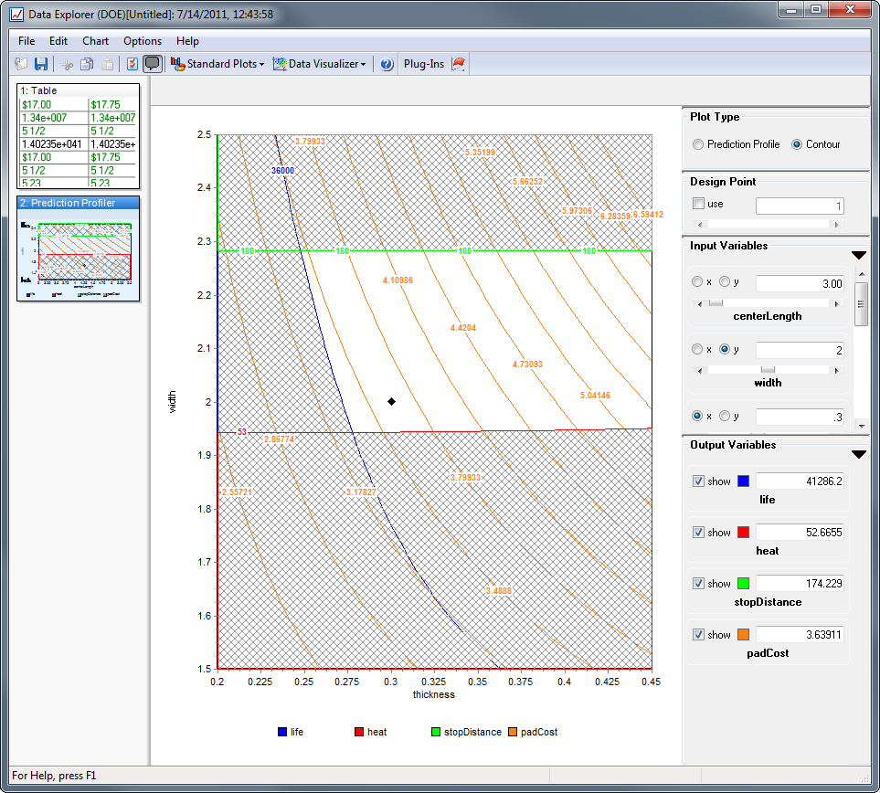
In the figure above, you can see the contour plot that is created by setting the lower bound for the life output variable to 36,000 and the upper bounds for the heat and stopDistance to 53 and 180 respectively. From the current design point (represented by the black diamond) the plot shows that it is possible to further reduce the cost without violating these constraints by decreasing the value of the width to 1.945 and thickness to .2775.

How does it Work?

The Prediction Profiler uses your data (or a portion of your data) to construct an approximate mathematical model of your product or process. Specifically, this mathematical model is an interpolating Kriging model. This model is used to predict the values of the output variables as a function of the input variables and to draw the profile and contour plots [1][2].

Recommendations

• Experimental design - The most accurate and reliable results will be obtained using a "space-filling" experimental design such as a Latin-Hypercube design, although any of the experimental designs available the DOE tool should be acceptable.
• Number of data points - As a general rule, use at least n(n+1)/2 points in your experimental design, where n is the number of design parameters that you wish to examine.

[1] Sacks, J., W.J. Welch, T.J. Mitchell, and H.P. Wynn, "Design and Analysis of Computer Experiments", Statistical Science, 4(4):409-435, 1989.

[2] Owen, A.B., "Orthogonal Arrays for Computer Experiments, Integration and Visualization", Statistica Sinica, 2:439-452, 1992.

The Prediction Profiler utilizes Boeing Design Explorer technology licensed to Ansys.