Probabilistic Analysis Tool Output

To view the Probabilistic Analysis Tool output, click on the View Output button. The Probabilistic Analysis Tool Output can be viewed at any time, and can be updated during the analysis run using the Refresh button. The Probabilistic Analysis Tool Output Dialog has five tabs, each displaying different information about the analysis run. Each page can be copied as an image and, if applicable, as text using the Copy button.

Basic Problem Setup

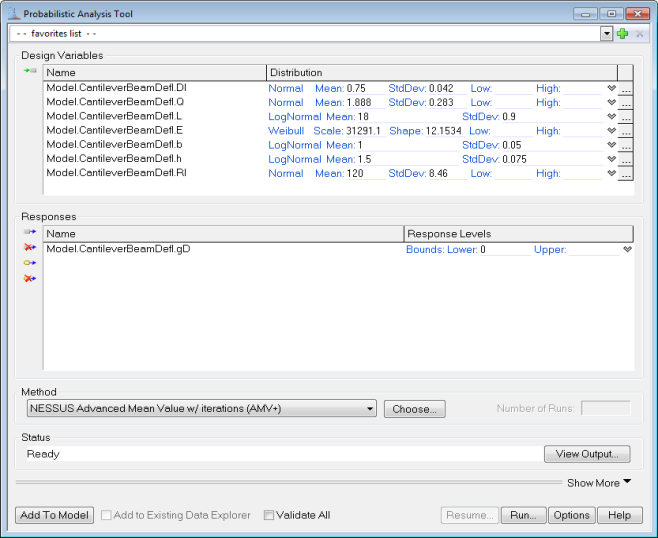
The basic problem setup under consideration is as above. This is an example of a simple cantilever beam under load Q at the free end. We are interested in determining the probability that the deflection at the free end is beyond the specified limit. The response variable Model.CantileverBeamDefl.gD denotes the limit state function for maximum deflection where gD < 0 denotes the failure region because gD = Deflection Limit - Maximum Deflection. Thus the probabilistic analysis is going to give us probability of failure of the cantilever beam under the deflection case. Thus 0 is set as the lower bound to denote that values less than 0 belong to the failure zone.

Results

The Results tab shows the probability of the response variable being less than specified Lower bound, which in this case is 0. Response variable Model.CantileverBeamDefl.gD being less than 0 actually represents the failure region, thus Probability of failure (pf) is 0.02651954. The Reliability is 0.97348. If there were multiple response variables in the problem setup, all of those will be listed in the Results tab. Since the current problem setup did not have an upper bound, the UB field is empty in the results table. If the Probabilistic Analysis Tool is added to the model, these pf and reliability values will be available in the component tree for further analysis. The values in the component tree can then be used as constraints or objective in the Optimization Tool if needed to perform reliability based design optimization.

Messages

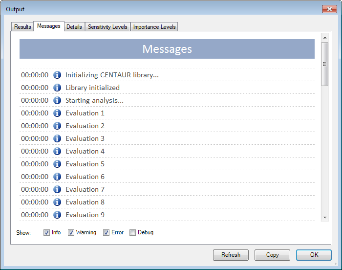
The Messages tab displays all of the messages that the probabilistic method generated while it was running. These are the same messages that get displayed in the Status area on the Probabilistic Analysis Tool form. This tab can be used to monitor the progress of the analysis and debug any failures. These messages can be filtered by message type:

– Info: Informational messages that indicate that the method is operating as expected
– Warn: Warning messages that indicate that something happened that might affect the results, but did not prevent the method from continuing
– Error: Error messages that indicate that an error occurred that prevented the method from continuing
– Debug: Debug messages that help in tracking down the causes of errors

Details

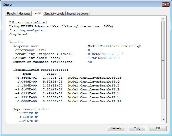
The Details tab displays a report generated by the method detailing the operations performed by the method during the analysis. The NESSUS methods give information about the probability that the Response variables are less than specified Lower bound or greater than the specified Upper bound. Thus in this case, the probability that gD is less than 0 (the performance level) is 0.0265195. The Reliability index (beta) is the shortest distance from the origin to the Most Probable Point (MPP) in transformed standard normal space. If the probability value is greater than 0.5 the value of beta will be negative. The Details tab also lists the number of model evaluations performed for each response variable. The probabilistic sensitivity levels and importance levels are also listed in the tab. These are the values used to create the plot in the Sensitivity Levels and Importance Levels tabs.

In some cases, the method will not be able to converge to a Most Probable Point and thus the results should not be considered valid. The individual method's help pages list the alternatives available in case of no convergence.

Sensitivity Levels [1]

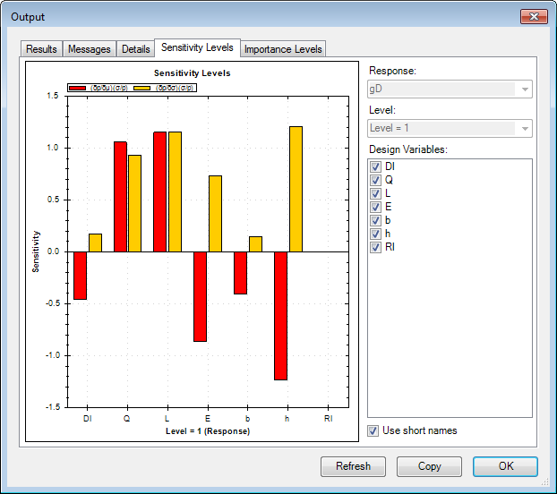
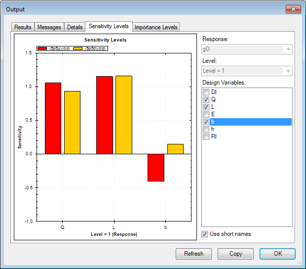
The Sensitivity Levels tab is displayed for all NESSUS methods i.e. methods other than Monte Carlo. The sensitivity levels plot shows how sensitive the response variable probability is to the parameters (mean or standard deviation) of each design variable. The red bars in the plot represent sensitivity with respect to the mean of each design variable. The yellow bars represent sensitivity with respect to the standard deviation of each design variable.

In probabilistic analysis, sensitivity is generally measured as the rate of change in probability relative to the change in mean or standard deviation of each design variable. Thus, looking at the plot above, it is clear that there is direct correlation between the standard deviation of each variable and the probability of failure because all the yellow bars are greater than 0. The relative heights of the yellow bars also mean that controlling standard deviation of design variables Dl (deflection limit) and b (width) is not going to lead to major reductions in the probability of failure. Hence, in order to reduce probability of failure, reducing the variation of design variables of L (length) and h (height) would yield appreciable results.

The red bars protruding into both positive and negative region indicate that reducing the mean for some variables would reduce the probability of failure, while reducing the mean for other variables would increase the probability of failure. For example, reducing the mean value of the design variables h (height) and E (modulus of elasticity) would increase the probability of failure. The plot also confirms the logical conclusion that a lower value of Q (load) or L (length of beam) would reduce the probability of failure as it would lead to lower deflection. These sensitivity levels can help to focus the engineer's attention and resources on those variables that have the most potential to reduce failures.

The sensitivity levels value is the rate of change of the probability with respect to the mean (or standard deviation) of the random variable and scaled by the ratio of the standard deviation of that variable to the computed probability. If the probability under consideration is greater than 0.5 then the denominator used for scaling is 1 - p instead of just p.

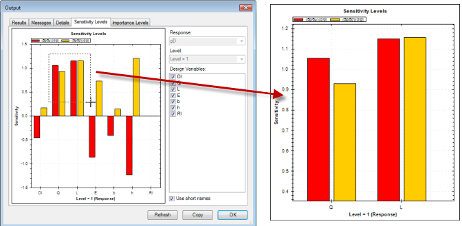
If there are only a few variables of interest, others can be deselected from the plot by using the Design Variable: section on the right hand side of the window. In the next screen, design variables Dl (Deflection limit), E (modulus of elasticity), h (Height) and Rl (Yield limit) were deselected from the plot.

Zooming can be accomplished by holding down on the left mouse button and dragging in the window plot area. A Right click in the plot area will bring up various options which can be used to zoom or un-zoom, copy, print or save the plot. The Use short names: checkbox can be used to make variable listing on the plot more readable.

If the probabilistic analysis had multiple response variables, there will be a different sensitivity levels plot for each response. In the following case, gY was added as the second response variable. This new variable is a limit state function for material yielding. A value less than 0 means that the beam has yielded beyond the specified limit and has therefore failed.

By selecting any particular response from the Response: drop down on the top right of the window, one can analyze individual sensitivity levels.

In this plot, one can infer that the probability of gD is insensitive to any change in the design variable Rl (yield limit). Similarly, gY is insensitive to any change in Dl (deflection limit) and E (modulus of elasticity). Again, from this new plot for gY, one can infer that increasing the variation of the design variables is not going to lead to any significant reduction of the probability of failure. In order to reduce the probability of failure for both cases, it would be beneficial to reduce the mean values of design variables Q and L. Similarly, increasing the mean values of design variables b and h would lead to a reduction in both probability of failures.

Importance Levels [1]

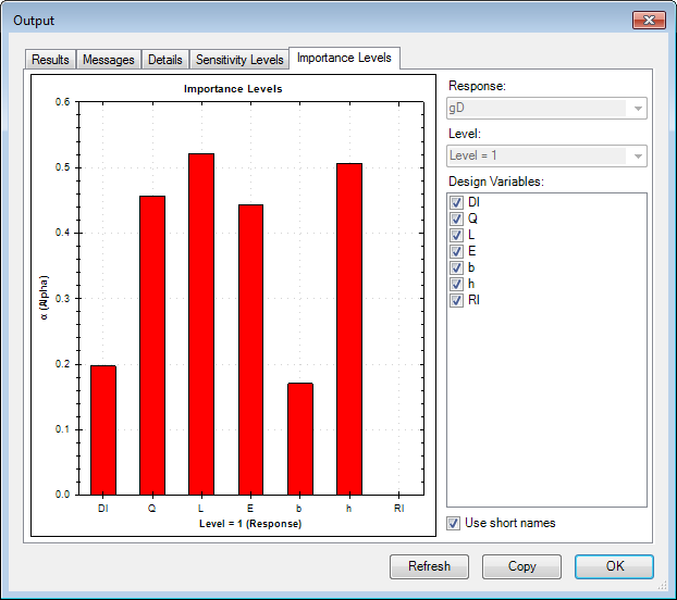
The Importance Levels tab is displayed for all NESSUS methods i.e. methods other than Monte Carlo. The Importance level is another good sensitivity measure because it illustrates the relative importance of the design variables. The taller the red bar, the more important that variable is. Thus it is evident that design variables Dl (deflection limit) and b (width) are relatively less important. This plot also shows that the design variable Rl is unimportant for the response variable gD.

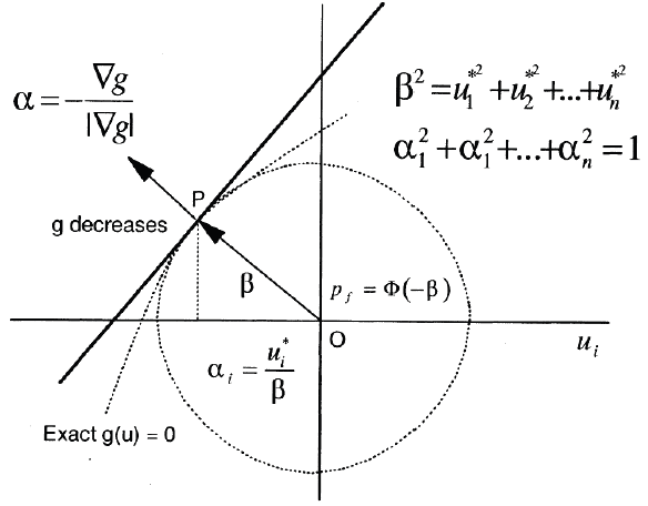
To compute the importance levels, the problem is transformed into standard normal u-space. The approximation of the limit state function is done and the MPP is found. The importance level is based on the location of the MPP (point P in the figure). At the MPP,

the first-order probability estimate is , where

Thus the unit normal vector at the MPP of the g = 0 (limit state function) surface is given as:

The alfa vector is positive towards the failure region i.e. it is directed towards decreasing values of g (limit state function). The directional cosines of the alfa vector which are projections on the respective u-axes are the Importance Levels values listed in the Details tab. The values shown in the Importance Levels plot are absolute values of those in Details tab. The directional cosines are given as:

If we were to square each of the directional cosines and add them they would add up to 1 and so squared values of Importance levels can be represented in a pie chart to show relative importance of design variables. The higher the value of Importance Levels (direction cosines), higher is the contribution of that variable to probability. Because the sensitivity analysis is based on the first-order reliability method, alfa is a good probability sensitivity measure only if is a good approximation to the true probability.

The controls/options on the Importance Levels tab are similar to those of Sensitivity Levels tab. A response variable can have a lower bound and upper bound specified, in which case the Probabilistic Analysis Tool will compute the probability between those two bounds as reliability. Suppose we want to know the probability of the response variable gD being greater than 0 but less than 0.5. The analytical methods will actually compute the probability of gD being less than 0 and then of being less than 0.5, then subtract the probability values to give us a reliability. Thus probability of failure will then be 1 - reliability. The random sampling methods do not care what the bounds are, they just compute probabilities once specified number of samples are done.

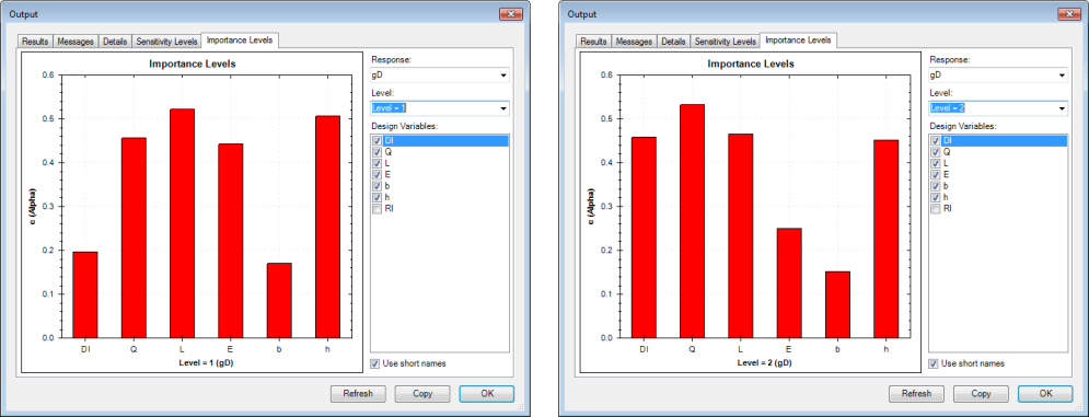
Importance levels will be available for both levels, i.e., lower bound and upper bound. This can be used to analyze how the impact of each design variable changes between those two bounds. Thus one can infer that the relative importance of Dl increases from the lower bound to the upper bound but that of E reduces.

Cumulative Distribution Function

The CDF tab is displayed for AMV+, FORM methods but only when the Response Levels option is "Generate a Cumulative Distribution Function (CDF)". The CDF tab is also displayed when more than one value is available for Probability Value or Performance Level type, but with the annotation that the plot may not be a full CDF. The CDF graph shows the total probability of each response occurring for any value it could possibly hold. The y-axis represents the cumulative probability, with values between 0 and 1 and the x-axis represents the values of the response variable. The CDF is useful tool to assess how a distribution fits the data because it measures the total probability as the value of the response changes, rather than the probability at certain point. The CDF plot can be used to gauge the range of the response variable.

In probabilistic analysis, the CDF is the probability that the measured variable takes a value less than or equal to x. Looking at the graph above, it is easy to see the range of values that gD can hold that will have a probability of it actually taking on that value. Probabilistic Analysis Tool uses 10 probability values listed here:

0.28716598E-06, 0.31688054E-04, 0.13496402E-02, 0.22747974E-01, 0.15864683, 0.84133901, 0.97724872, 0.99864996, 0.99996831, & 0.99999971

It then uses the method to compute corresponding response values. Using the "Input" and "Output" array linking feature on the main PAT window, the CDF probability values and response values can be updated into array variables.

The controls/options on the CDF tab are very straightforward. Each response ran with the method will have its own CDF generated. The dropdown menu labeled "Response:"controls which variable's CDF is currently displayed. It is important to note that a CDF will only be generated if "Response Levels"tab from the Probabilistic Analysis Tool window has the option "Generate a Cumulative Distribution Function (CDF)"selected. The CDF plot is also used to plot real probability values when you have selected "Performance Levels"or "Probability Levels". In both these cases the plot does not show a CDF but just plots probability values against response values.

References: 1. NESSUS Theoretical Manual, February 17, 2012, Section 2.6