STK Premium (Space) or STK Enterprise
You can obtain the necessary licenses for this tutorial by
The results of the tutorial may vary depending on the user settings and data enabled (online operations, terrain server, dynamic Earth data, etc.). It is acceptable to have different results.
Capabilities covered
This lesson covers the following capabilities of the Ansys Systems Tool Kit® (STK®) digital mission engineering software:
- STK Pro
- Astrogator
- Analysis Workbench
Problem statement
Engineers and operators require a quick way to design high-fidelity spacecraft trajectories for mission planning and operations. You want to design a maneuver from an initial state to the Sun-Earth libration (or Lagrange) point, L1.
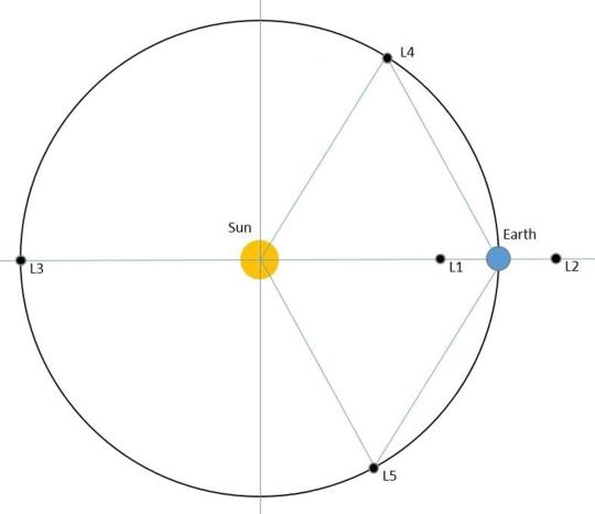
Libration points in the Sun-Earth system
Solution
Use the STK/Astrogator® and Analysis Workbench capabilities to build and propagate the various sequences of launching a spacecraft to a libration point orbit around the Sun-Earth libration point. The goal of this tutorial is to model a mission to the vicinity of the L1 point.
What you will learn
Upon completion of this tutorial, you will be able to:
- Create custom geometry and calculation objects for libration points
- Configure the magnitude of the injection thrust
- Understand the effects of perturbations on the mission
- Model orbital station-keeping at the Sun-Earth libration point, L1
Video guidance
Watch the following video. Then follow the steps below, which incorporate the systems and missions you work on (sample inputs provided).
Creating a new scenario
First, you must create a new scenario, and then build from there.
- Launch the STK application (
 ).
). - Click
 Create a Scenario when the Welcome to STK dialog box opens.
 - Enter the following in the STK: New Scenario Wizard:
- Click when you finish.
- Click Save (
 ) when the scenario loads. The STK software creates a folder with the same name as your scenario for you.
 - Verify the scenario name and location in the Save As dialog box.
- Click .
| Option | Value |
|---|---|
| Name | Sun_Earth_L1 |
| Start | 15 Jan 2025 00:00:00.000 UTCG |
| Stop | 15 Aug 2026 00:00:00.000 UTCG |
Save (![]() ) often during this scenario!
) often during this scenario!
Modeling the Sun, Earth, and Moon
A
Adding the Planet object to the Insert STK Objects tool
You must first add the Planet object to the Insert STK Objects tool to be able to add them into your scenario.
- Bring the Insert STK Objects tool (
 ) to the front.
 - Click in the Insert STK Objects tool.
- Ensure the New Object page is selected when the Preferences dialog box opens.
- Select the Show check box for the Planet option in the Define Default Creation Methods frame.
- Click to accept your selection and to close the Preferences dialog box.
Inserting Planet objects into the scenario
Start by inserting three Planet objects to model the Sun, Earth and Moon.
- Select Planet (
 ) in the Select An Object To Be Inserted list.
 - Select Insert Default () in the Select A Method list.
- Click three times to insert three Planet objects.
Modeling the Sun
The options on the
- Right-click on Planet1 () in the Object Browser.
- Select Properties (
 ) in the shortcut menu.
 - Select the Basic - Definition page when the Properties Browser opens.
- Note the Central Body selection is Sun by default.
- Click to accept your selection and to close the Properties Browser.
Note the name of the Planet object was automatically updated to Sun when you clicked .
Selecting the Earth
Select Earth as the central body of the second Planet object.
- Open Planet2's () Properties ().
- Select the Basic - Definition page.
- Open the Central Body drop-down list.
- Select Earth.
- Click to accept your selection and to close the Properties Browser.
Note the Ephemeris Source is set to Default.
Note the name of the Planet object was automatically updated to Earth.
Selecting the Moon
Select the Moon as the central body of the third planet object.
- Open Planet3's () Properties ().
- Select the Basic - Definition page.
- Open the Central Body drop-down list.
- Select Moon.
- Click to accept your selection and to close the Properties Browser.
Note the name of the Planet object was automatically updated to Moon.
Configuring the 2D and 3D Graphics windows
The
Setting the display options
Configure the scenario's global 2D Graphics attributes to visualize the orbit tracks of the planets in relation to the L1 point. You can choose to have individual objects inherit these attributes from the scenario or you can override these options in the object's properties. By definition, overridable attributes are global.
- Open Sun_Earth_L1's () Properties ().
- Select the 2D Graphics - Global Attributes page.
- Set the following options in the Planets panel:
- Click to accept your changes and to close the Properties Browser.
| Option | Value |
|---|---|
| Show Orbits | Selected |
| Show Inertial Positions | Selected |
| Show Position Labels | Selected |
| Show Subplanet Points | Clear |
| Show Subplanet Labels | Clear |
Configuring the 3D Graphics window properties
The STK application displays complex scenario information in an intuitive 3D environment. This environment can display complex mission and orbit geometries, realistic 3D views of airborne and terrestrial assets, sensor projections, and orbit trajectories. The 3D graphics engine is driven by validated numerical data. To view a scenario in 3D, place a virtual camera among the objects in the scenario using the
- Bring the 3D Graphics window to the front.
- Click Properties () in the 3D Graphics window toolbar.
- Select the Advanced page when the Properties Browser opens.
- Enter 1e+12 km in the Max Visible Distance field.
- Enter 55 deg in the Field of View field.
- Click to accept your changes and to close the Properties Browser.
The default value is 10 million (1e+07) kilometers.
The Field of View specifies how wide of an angle you can see, in degrees, in the 3D Graphics window. The larger the value, the more you can see. The maximum angle is 160 degrees. A large field of view is similar to a wide-angle lens in photography, where size differences are exaggerated due to proximity to the camera. A small field of view is similar to a telescopic lens.
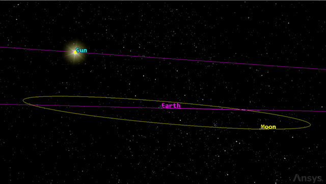
3D graphics view of the Sun, Earth, and Moon
Configuring an orthographic projection in the 2D Graphics window
The
- Bring the 2D Graphics window to the front.
- Click Properties () on the 2D Graphics window toolbar.
- Select the Projection page.
- Open the Type drop-down list in the Projection Format panel.
- Select Orthographic.
- Open the Display Coordinate Frame drop-down list.
- Select BBR.
- Enter 2e+06 km in the Display Height field.
BBR stands for Body-to-body Rotating. If you choose BBR, use the Secondary Body option to select a secondary celestial body. This list may include asteroids and other celestial bodies in addition to the planets typically available in the STK application.
Note the Secondary Body selection defaults to Sun.
When you select the orthographic map projection, you can specify the height of the viewing plane. In all cases, the observer's position is fixed in the ECF reference frame at the Projection Center Position.
Displaying and formatting the axes for the orthographic projection
After selecting the Orthographic projection type,
- Select the Show Axes check box to show the X, Y, and Z axes for that view.
- Click .
- Open the Coordinate Frame drop-down list when the Format Axes dialog box opens.
- Select BBR.
- Use the default Sun selection for the Secondary Body.
- Open the +X Axis Color drop-down list.
- Select yellow.
- Enter 250 in the +X Axis Scale field.
- Click to accept your changes and to close the Format Axes dialog box.
Selecting the orthographic projection's center point
Use the options in the Center panel to select the center point for the map projection on the North Pole. Enter the exact latitude and longitude degrees in the respective fields.
- Enter the following in the Center panel:
- Click to accept your changes and to close the Properties Browser.
| Option | Value |
|---|---|
| Lat | 90 deg |
| Lon | 90 deg |
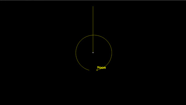
2D graphics orthographic projection
Creating custom geometry components for the L1 point
Create and display the proper geometry for the L1 point using the Analysis Workbench capability's
Selecting the central body
Set the Sun to be the primary central body of your VGT component.
- Right-click on Sun_Earth_L1 () in the Object Browser.
- Select Analysis Workbench... (
 ) in the shortcut menu.
 - Select the Vector Geometry tab in the Analysis Workbench.
- Open the Filter by drop-down list.
- Select Primary Central Bodies.
- Select Sun (
 ) in the object tree.
Creating an assembled system
A System component defines location and translation motion of the origin orientation, and rotational motion of a triad of mutually orthogonal uni vectors in three-dimensional space. An assembled system is a system composed of an origin point and a set of reference axes.
- Click Create new System (
 ) in the Vector Geometry toolbar.
 - Keep the default Assembled type when the Add Geometry Component dialog box opens.
- Enter Syst_SEM_L1 in the Name field.
Selecting the origin point
Add the SEM_L1 libration point as the reference point for the system. The SEM acronym denotes Sun, Earth-Moon. The corresponding L1 point is the interior collinear libration point associated with the system comprised of the Sun and the Earth-Moon barycenter.
- Click the Origin Point ellipsis (
 ).
). - Select Sun () in the object tree when the Select Reference Point dialog box opens.
- Select SEM_L1 (
 ) in the Points for: Sun list.
 - Click to accept your selections and to close the Select Reference Point dialog box.
Selecting the reference axes
Select the SEM_L1 axes for the reference axes. The SEM axes are the central-body aligned axes of the selected libration point between one primary and multiple secondary central bodies, with the X axis along the position of the libration point relative to the primary center of mass and the Z axis along the orbit normal of the libration point relative to the primary center of mass.
- Click the Reference Axes ellipsis ().
- Select Sun () in the object tree when the Select Reference Axes dialog box opens.
- Select SEM_L1 (
 ) in the Axes for: Sun list.
 - Click to accept your selections and to close the Select Reference Axes dialog box.
- Click to accept your selections and to close the Add Geometry Component dialog box.
Displaying geometry components in the 3D Graphics window
Configure your custom planes for display in the 3D Graphics window.
Displaying the Syst_SEM_L1 planes
You can control the display of geometric elements related to central bodies using the
- Bring the 3D Graphics window to the front.
- Click Properties () in the 3D Graphics window toolbar.
- Select the Vector page when the Properties Browser opens.
- Select the Planes tab.
- Click .
- Select Sun () in the object tree when the Add Components dialog box opens.
- Expand (
 ) Syst_SEM_L1 () in the Components for: Sun list.
 - Using the CTRL key, multi-select both the YZ (
 ) and XZ () planes.
 - Click to accept your selections and to close the Add Components dialog box.
Configuring the Y-Z plane
Change the view and scale for the Y-Z plane.
- Double click the Color cell for Sun Syst_Sem_L1.YZ Plane.
- Open the Color drop-down list.
- Select gray.
- Clear the Draw at object check box.
- Select the Translucent plane check box to make the plane semi-transparent.
- Enter 50 in the Scale field in the Component Size panel of the Common Options panel.
Set the scale to 50 since the scenario deals with very large distances.
Configuring the X-Z plane
Change the view and scale for the X-Z plane.
- Double click the Color cell for Sun Syst_Sem_L1.XZ Plane.
- Open the Color drop-down list.
- Select gray.
- Clear the Draw at object check box.
- Select the Translucent plane check box.
- Click to accept your changes and to keep the Properties Browser open.
Viewing the planes in the 3D Graphics window
Review your changes in the 3D graphics window.
- Bring the 3D Graphics window to the front.
- Use your mouse to view the planes and the L1 point.
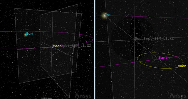
L1 Y-Z and X-Z planes
You now see the two planes are displayed at the L1 point.
Creating a second assembled system
The strategy you will use to launch from an initial state to the L1 point is a ballistic transfer from the defined low Earth orbit. The first burn will happen when the probe intersects the anti-Sun line for a proper alignment. The anti-Sun line joins the Sun and Earth as it extends through and beyond the Earth from the umbra side.
Creating a new system
To better understand the geometry, create a new assembled System component using the VGT.
- Return to the Analysis Workbench.
- Select the Vector Geometry tab.
- Select Earth () in the object tree when the Add Geometry Component dialog box opens.
- Click Create new System () in the Vector Geometry toolbar.
- Keep Assembled as the default type.
- Enter L1_LEO in the Name field.
Selecting the origin point
Add the Earth Center point as the reference point for the system.
- Click the Origin Point ellipsis ().
- Select Earth () in the object tree when the Select Reference Point dialog box opens.
- Select Center (
 ) in the Points for: Earth list.
 - Click to accept your selections and to close the Select Reference Point dialog box.
Selecting the reference axes
Select the SEM_L1 axes for the reference axes.
- Click the Reference Axes ellipsis ().
- Select Sun () in the object tree when the Select Reference Axes dialog box opens.
- Select SEM_L1 (
 ) in the Axes for: Sun list.
 - Click to accept your selections and to close the Select Reference Axes dialog box.
- Click to accept your selections and to close the Add Geometry Component dialog box.
Adding the custom axes to the 3D Graphics window
Add the Earth L1_LEO system's axes for display in the 3D Graphics window
- Bring the 3D Graphics window to the front.
- Click Properties () in the 3D Graphics window toolbar.
- Select the Vector page when the Properties Browser opens.
- Select the Axes tab.
- Click .
- Select Earth () in the object tree when the Add Components dialog box opens.
- Extend () L1_LEO () in the Components for: Earth list.
- Select Axes ().
- Click to accept your selections and to close the Add Components dialog box.
Adding the custom plane to the 3D Graphics window
Add the Earth L1_LEO system's XY plane to the 3D Graphics window.
- Select the Planes tab.
- Click .
- Select Earth () in the object tree when the Add Components dialog box opens.
- Expand () L1_LEO () in the Components for: Earth list.
- Select XY ().
- Click to accept your selections and to close the Add Components dialog box.
Updating the plane's display
Change the color and transparency of the Earth L1_LEO.XY Plane.
- Double click on the Earth L1_LEO.XY Plane color cell.
- Open the Color drop-down list.
- Select yellow.
- Clear the Draw at object check box.
- Select the Translucent plane check box.
- Click to accept your changes and to close the Properties Browser.
Viewing the custom plane and axes in the 3D Graphics window
The newly added plane is the reference and the stopping condition for the initial (coasting) spacecraft propagation. View your changes in the 3D Graphics window.
- Bring the 3D Graphics window to the front.
- Use your mouse to obtain situational awareness of the plane and axes.
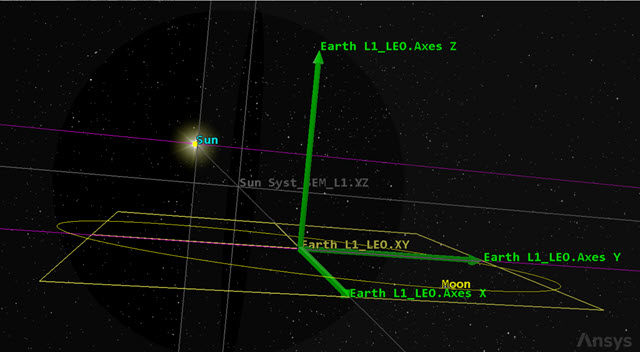
custom axes and plane
Modeling the orbit injection maneuver
Use a Satellite object to model the probe and configure a Mission Control Sequence to model the maneuver to reach the L1 point.
Inserting a Satellite object
Insert a Satellite object and name it L1_Probe.
- Bring the Insert STK Objects tool () to the front.
- Insert a Satellite (
 ) object using the Insert Default () method.
 - Right-click on Satellite1 () in the Object Browser.
- Select Rename in the shortcut menu.
- Rename Satellite1 () L1_Probe.
Setting L1_Probe's orbit tracks
The display of leading and trailing portions of a route, ground track, trajectory or orbit is determined on the basis of the current animation time. A lead type of All displays the track spanning the entire vehicle ephemeris.
- Open L1_Probe's () Properties ().
- Select the 2D Graphics - Pass page when the Properties Browser opens.
- Open the Lead Type drop-down list in the Orbit Track panel.
- Select All.
- Select the 3D Graphics - Pass page.
- Open the Lead Type drop-down list in the Orbit Track panel.
- Select All.
- Click to accept your changes and to keep the Properties Browser open.
Selecting a trajectory frame
Set the BBR orbit system for the L1_Probe to display in the 3D Graphics window on the
- Select the 3D Graphics - Orbit System page.
- Select 3D Graphics 1 - Earth in the 3D Windows panel list.
- Click .
- Keep Earth as the Primary Central Body when the Select BBR Orbit System dialog box opens.
- Open the Secondary Central Body drop-down list.
- Select Sun.
- Click to accept your selection and to close the Select BBR Orbit System dialog box.
- Clear the Show check box for the Inertial by Window system in the System list.
- Click to accept your changes and to keep the Properties Browser open.
Changing the propagator to Astrogator
The Astrogator capability contains specialized analysis for interactive orbit maneuver and spacecraft trajectory design. Astrogator acts as one of the propagators available for a Satellite object. Astrogator calculates the Satellite's ephemeris by running a Mission Control Sequence, or MCS, that you define according to the requirements of your mission.
- Select the Basic - Orbit page.
- Open the Propagator drop-down list.
- Select Astrogator.
Adding a Target Sequence
The
Add a
- Right-click on the Return (
 ) segment in the MCS.
 - Select Insert Before... in the shortcut menu.
- Select Target Sequence (
 ) when the Segment Selection dialog box opens.
 - Click to accept your selection and to close the Segment Selection dialog box.
- Right-click on Target Sequence () in the MCS.
- Select Rename in the shortcut menu.
- Rename Target Sequence () Target Plane Crossing.
- Click and drag the Initial State (
 ) segment and nest it in the Target Plane Crossing () Target Sequence.
 - Click and drag the Propagate (
 ) segment and nest it in the Target Plane Crossing () Target Sequence below the Initial State () segment.
Note that Target Plane Crossing (![]() ) has automatically been renamed Target_Plane_Crossing (
) has automatically been renamed Target_Plane_Crossing (![]() ).
).
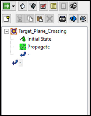
MCS view
Your MCS should look like the image above.
Defining the Initial State segment
Use the
- Select Initial State () in the MCS.
- Select the Elements tab.
- Open the Coordinate Type drop-down list.
- Select Keplerian.
- Make sure the Orbit Epoch matches your scenario start time of 15 Jan 2025 00:00:00.000 UTCG.
- Enter 0 in the Eccentricity field.
- Use the Right Asc. of Asc. Node (the RAAN) as a control parameter (independent variable) by clicking its target icon. A check mark appears over the target.
- Keep the rest of the default settings.
By selecting the RAAN as an independent variable, you are telling Astrogator to determine the value for you later on when you run the MCS.
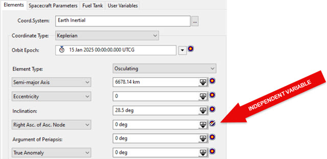
orbital parameters
Defining the Propagate segment
Use the
- Right-click on Propagate () in the MCS.
- Select Rename in the shortcut menu.
- Rename Propagate () Coast.
Adding a new stopping condition
Use the X-Y Plane Cross
- Click New... (
 ) in the Stopping Conditions panel toolbar.
 - Select X-Y Plane Cross (
 ) when the New Stopping Condition dialog box opens.
 - Click to accept your selection and to close the New Stopping Condition dialog box.
- Select the Duration stopping condition.
- Click Delete (
 ) in the Stopping Conditions panel toolbar.
Setting the X-Y Plane Cross parameters
Use the custom coordinate system that you created and set the Criterion for the Stopping Condition to Cross Decreasing. Cross Decreasing means the stopping condition is satisfied when the parameter reaches a value equal to the trip value while decreasing.
- Click the Coord. System ellipsis ().
- Select Earth () in the object tree when the Select Reference dialog box opens.
- Select L1_LEO (
 ) in the System for: Earth list.
 - Click to accept your selection and to close the Select Reference dialog box.
- Open the Criterion drop-down list.
- Select Cross Decreasing.
- Click to accept your changes and to keep the Properties Browser open.
Adding a result
Recall that you selected the RAAN as an independent variable when setting up the initial state. Select that component as the result for the Coast Propagate segment's stopping condition.
- Click .
- Expand () the Spherical Elems (
 ) folder in the Available Components list when the User-Selected Results - Coast dialog box opens.
 - Select Right Asc ().
- Click Insert Component (
 ).
). - Double-click Earth Inertial in the Value cell in the Component Details list.
- Select Earth () in the object tree when the Select Reference dialog box opens.
- Select L1_LEO () in the Systems for: Earth list.
- Click to accept your selection and to close the Select Reference dialog box.
- Click to accept your selections and to close the User-Selected Results - Coast dialog box.
- Click to accept your changes and to keep the Properties Browser open.
Defining the Differential Corrector
The
- Select Target_Plane_Crossing () in the MCS.
- Click twice in the Differential Corrector cell in the Profiles panel and wait until the text is highlighted.
- Enter Anti-Sun Line in the Name cell.
Setting the Differential Corrector properties
In order to match the anti-Sun line when crossing the L1_LEO X-Y plane, you need to null the RAAN in the Earth L1_LEO reference system.
- Click Properties... () in the Profiles panel toolbar.
- Select the Use check box for InitialState.Keplerian.RAAN in the Control Parameters panel when the Anti-Sun Line dialog box opens.
- Select the Use check box for Right_Asc in the Equality Constraints (Results) panel.
- Click to accept your selections and to close the Anti_Sun Line dialog box.
Earlier, when you clicked on the Initial State target, you set the RAAN as the control parameter. You want Astrogator to determine this value.
The is the result you selected for the Propagate segment.
Running the Mission Control Sequence
To calculate the trajectory of the spacecraft you must run the Mission Control Sequence. Astrogator will proceed through the MCS and run each segment, generating an ephemeris for the spacecraft. As it runs the MCS, Astrogator carries the trajectory and state of the spacecraft determined so far from one segment to the next.
- Open the Action drop-down list.
- Select Run active profiles.
- Click Run Entire Mission Control Sequence (
 ) the MCS toolbar.
 - Look at the Targeting Status window.
- Close (
 ) the Target Status window.
 - Click in the Profiles and Corrections panel.
- Click Clear Graphics (
 ) in the MCS toolbar.
 - Click to accept your changes and to keep the Properties Browser open.
The Run Active profiles option runs the Mission Control Sequence allowing the active profiles to operate.
It should say *CONVERGED* and also provide data on the run.
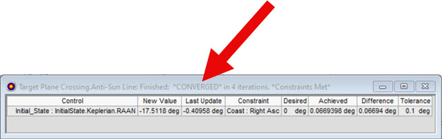
targeting status window
This applies the values of the search profile's controls and the changes specified by the segment configuration profiles to the segments within the target sequence.
Reviewing the changes to the Initial State segment
You previously had selected the RAAN as an independent variable. Review the changes to that value in the Initial State segment.
- Select Initial State () in the MCS.
- Select the Elements tab.
- Look at the value of the Right Asc. of Asc. Node.
The default value was 0. After running the Mission Control Sequence and applying the changes, you should see the new RAAN value, for example, 342.488 deg.
Viewing the orbit in the 3D Graphics window
You can view the orbit as it stops at the anti-sun line in the 3D Graphics window.
- Bring the 3D Graphics window to the front.
- Click Home View (
 ) in the 3D Graphics toolbar.
 - Use your mouse to obtain situational awareness of L1_Probe's () orbit and where it stops at the anti-sun line.
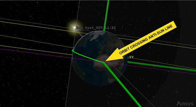
orbit crossing anti-sun line
The probe now crosses the X-Y L1_LEO plane exactly in the anti-Sun line direction. This gives you the opportunity to burn for the transfer orbit with the correct geometry.
Defining the Maneuver segment
Use an
- Select Coast () in the MCS.
- Click Insert Segment After () in the MCS toolbar.
- Select Maneuver (
 ) when the Segment Selection dialog box opens.
 - Click to accept your selection and to close the Segment Selection dialog box.
- Click Segment Properties () in the MCS toolbar.
- Enter L1 LEO Injection Thrust in the Name field when the Edit Segment dialog box opens.
- Open the Color drop-down list.
- Select white.
- Click to accept your changes and to close the Edit Segment dialog box.
An impulsive maneuver type can't be seen in the 2D and 3D Graphics windows. You can change the color to white in the MCS to make it stand out as an impulsive maneuver type.
Defining a second Propagate segment
You need to add another Propagate segment and set the stopping condition to model the probe's state after the burn.
- Select L1 LEO Injection Thrust () in the MCS.
- Click Insert Segment After () in the MCS toolbar.
- Select Propagate () when the Segment Selection dialog box opens.
- Click to accept your selection and to close the Segment Selection dialog box.
- Click Segment Properties () in the MCS toolbar.
- Enter Z-X Plane Crossing in the Name field when the Edit Segment dialog box opens.
- Open the Color drop-down list.
- Select a color that is different from Coast ().
- Click to accept your changes and to close the Edit Segment dialog box.
Unlike an impulsive maneuver type, Propagate segments can be seen in the 2D and 3D Graphics windows.
Selecting a new stopping condition
Apply a Z-X Plane Cross stopping condition, which stops the propagation when it crosses the X-Z plane that is located along the Sun-Earth direction.
- Click New... () in the Stopping Conditions panel toolbar.
- Select Z-X Plane Cross () when the New Stopping Condition dialog box opens.
- Click to accept your selection and to close the New Stopping Condition dialog box.
- Select the Duration stopping condition.
- Click Delete () in the Stopping Conditions panel toolbar.
Setting the stopping condition parameters
Change the stopping condition propagator to Cislunar. The L1 Probe is operating in cislunar space with motion governed by both the gravity of the Earth and of the Moon, each to relatively comparable effect.
- Click the Propagator ellipsis ().
- Select Cislunar () when the Select Component dialog box opens.
- Click to accept your selection and to close the Select Component dialog box.
- Click .
- Enter 864000 sec in the Minimum Propagation Time field when the Propagator Advanced dialog box opens.
- Click to accept your change and to close the Propagator Advanced dialog box.
This is equivalent to 10 days.
Updating the Coordinate System
Use the custom SEM_L1 coordinate system for the Propagate segment.
- Click the Coord. System ellipsis ().
- Select Sun () in the object tree in the Select Reference dialog box.
- Select Syst_SEM_L1 () in the Systems for: Sun list.
- Click to accept your selection and to close the Select Reference dialog box.
- Click to accept your changes and to keep the Properties Browser open.
Guessing a thrust vector velocity
You can apply a first guess for the magnitude of the thrust to correctly put the probe in orbit around the L1point. You'll try some values manually and then use the Differential Corrector to find the exact value.
- Select L1 LEO Injection Thrust () in the MCS.
- Select the Attitude tab.
- Open the Attitude Control drop-down list.
- Select Thrust Vector.
- Enter 3160.00 m/sec in the X (Velocity) field.
- Click to accept your changes and to keep the Properties Browser open.
- Click Run Entire Mission Control Sequence () the MCS toolbar.
- Bring the 2D Graphics window to the front.
2D Graphics window first guess
This magnitude is not sufficient to reach L1_LEO. The L1_Probe is attracted back toward Earth.
Increasing the probe's velocity
Make another guess, this time, increasing the velocity to 3,170.00 m/sec.
- Return to L1_Probe's () Properties ().
- Enter 3170.00 m/sec in the X (Velocity) field.
- Click to accept your change and to keep the Properties Browser open.
- Click Run Entire Mission Control Sequence () the MCS toolbar.
- Bring the 2D Graphics window to the front.
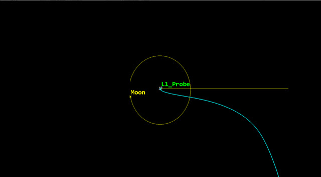
2D Graphics window Second guess
This time you overshot and the L1_Probe moves away from the L1 point.
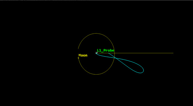
Making a third guess
You set the X (Velocity) to 3,160 m/sec first and didn't reach L1_LEO. Then you set the X (Velocity) to 3,170 m/sec and missed the L1 point completely. You could keep guessing. Try an X (Velocity) that gets you close to the L1Point
- Return to L1_Probe's () Properties ().
- Set the X (Velocity) to 3167.1 m/sec.
- Click to accept your change and to keep the Properties Browser open.
- Click Run Entire Mission Control Sequence () the MCS toolbar.
- Bring the 2D Graphics window to the front.
2D Graphics window third guess
This is a good guess for the Delta-V. Considering the target is the L1 region, you see how the final condition is very sensitive to changes in Delta-V.
Creating a custom Calculation Object component
You can set up a second Differential Corrector to get a better burn magnitude estimate. For this purpose, you can use the Cartesian SEM L1 X velocity (Vx) as the constraint. You want to cross the X-Z plane with a SEM L1 Vx = 0 km/sec. That value should guarantee that you have another X-Z plane crossing.
You can use a
- Return to L1_Probe's () Properties ().
- Click Component Browser (
 ) in the MCS toolbar.
 - Expand () the Calculation Objects () folder in the Show Component Type list when the Component Browser opens.
- Select Cartesian Elems ().
- Select Vx () in the Cartesian Elems list.
- Click Duplicate component (
 ) in the Cartesian Elems toolbar.
 - Enter VxL1 in the Name field of the Field Editor dialog box.
- Click to accept your changes and to close the Field Editor dialog box.
Updating VxL1's parameters
To ensure the L1_Probe remains near the L1 point, the X component of the velocity needs to be nearly zero at the Rotating Libration Point (RLP) X-Z plane crossing.
- Double-click on VxL1 (
 ).
). - Double-click in the CoordSystem row when the Inertial in the Cartesian Elem - VxL1 dialog box opens.
- Select Sun () in the object tree when the Select Reference dialog box opens.
- Select Syst_SEM_L1 () in the Systems for: Sun list.
- Click to accept your selection and to close the Select Reference dialog box.
- Click to close the Cartesian Elem - VxL1 dialog box.
- Click to close the Component Browser.
Setting VxL1 as a result
You can apply the VxL1 component as a Propagation segment result.
- Return to L1_Probe's () Properties ().
- Select Z-X Plane Crossing () in the MCS.
- Click .
- Expand () the Cartesian Elems () folder in the Available Components list when the User-Selected Results - Z-X Plane Crossing dialog box opens.
- Select VxL1 ().
- Click Insert Component ().
- Click to accept your selection and to close the User-Selected Results - Z-X Plane Crossing dialog box.
Selecting L1 LEO Injection's X (Velocity) as a control parameter
With your Calculation object in place, select X (Velocity) as an additional independent variable.
- Select L1 LEO Injection () in the MCS.
- Select the Attitude tab.
- Click the X (Velocity) target (
 ) to make it a control parameter.
Adding a new Differential Corrector
Add a second Differential Corrector to the Target Plane Crossing Target Sequence.
- Select Target Plane Crossing () in the MCS.
- Click New... () in the Profiles panel toolbar.
- Select Differential Corrector () when the New... dialog box opens.
- Click to accept your selection and to close the New... dialog box.
- Click twice on the Differential Corrector cell in the Profiles panel and wait until the text is highlighted.
- Enter First Plane Crossing in the Name cell.
- Select the Enter key.
Updating First Plane Crossing's properties
Select the X (Velocity) control parameter and the VxL1 component as the result.
- Click Properties... () in the Profiles panel toolbar.
- Select the Use check box for ImpulsiveMnvr.Pointing.Cartesian.X in the Control Parameters panel when the First Plane Crossing dialog box opens.
- Select the Use check box for VxL1 in the Equality Constraints (Results) panel.
- Click to accept your selections and to close the First Plane Crossing dialog box.
- Click to accept your changes and to keep the Properties Browser open.
Running the Mission Control Sequence
With your differential correctors set, re-run your Mission Control Sequence.
- Click Run Entire Mission Control Sequence () in the MCS toolbar.
- Click Clear Graphics () in the MCS toolbar.
- Click to accept your changes and to keep the Properties Browser open.
- Click the in the Profiles and Corrections panel.
- Select L1 LEO Injection () In the MCS.
- Notice that the X (Velocity) value has changed since your last guess.
The converged Delta-V value (for example, 3167.15 m/sec) should be very close to the guess you made.
Creating a Libration Point Orbit (LPO)
The SEM L1 region has a large degree of instability. The instability might mean the spacecraft requires only very small maneuvers to maintain its desired path.
Duplicating the Propagate segment
Copy the Z-X Plane Crossing Propagate segment to view the orbital instability.
- Select Z-X Plane Crossing () in the MCS.
- Click Copy (
 ) in the MCS toolbar.
 - Right-click on the bottom Return () segment in the MCS.
- Select Paste Before in the shortcut menu.
- Click Segment Properties () in the MCS toolbar.
- Enter LPO in the Name field when the Edit Segment dialog box opens.
- Open the Color drop-down list.
- Select a color that is different for the other Propagate segments.
- Click to accept your changes and to close the Edit Segment dialog box.
- Click to accept your changes and to keep the Properties Browser open.
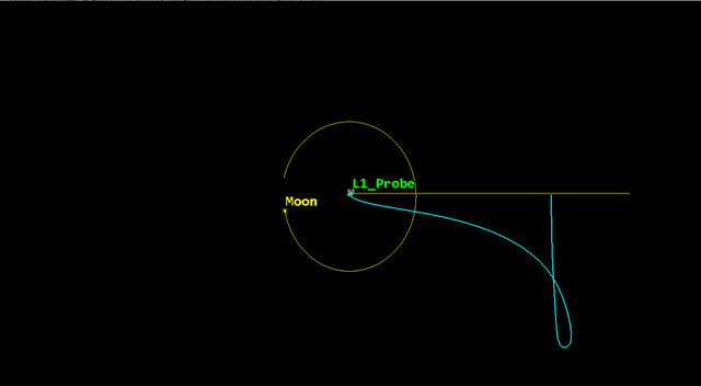
Running the Mission Control Sequence
Re-run the entire Mission Control Sequence with your additional Propagate segment.
- Click Run Entire Mission Control Sequence () in the MCS toolbar.
- Click Clear Graphics () in the MCS toolbar.
- Click to accept your changes and to keep the Properties Browser open.
- Bring the 2D Graphics window to the front.
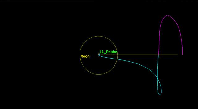
first libration point maneuver
Without a small injection maneuver, the probe returns to the Earth. It follows a somewhat symmetric path with respect to the Sun-Earth line.
Perturbing the trajectory into orbit
You would like to ensure the probe begins to orbit about the L1 point. To do this, modify the MCS to favorably perturb the trajectory toward orbital motion.
- Return to L1_Probe's () Properties ().
- Select Target Plane Crossing () in the MCS.
- Select First Plane Crossing in the Profiles panel.
- Click Properties... () in the Profiles panel toolbar.
- Double click the VxL1 Desired Value cell in the Equality Constraints (Results) list of the First Plane Crossing dialog box.
- Enter -0.01 km/sec.
- Click to accept your change and to close the First Plane Crossing dialog box.
Running the Mission Control Sequence
Re-run your Mission Control Sequence to view the effects of the perturbation.
- Click Run Entire Mission Control Sequence () in the MCS toolbar.
- Click Clear Graphics () in the MCS toolbar.
- Click to accept your changes and to keep the Properties Browser open.
- Bring the 2D Graphics window to the front.
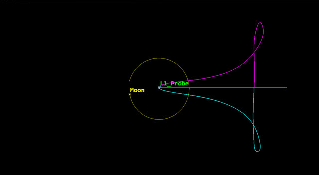
Second libration point maneuver
You should now see a sufficient amount of drift for the trajectory to start orbiting around the L1 point.
Adding a new stopping condition
Add a new stopping condition to the LPO Propagate segment.
- Return to L1_Probe's () Properties ().
- Select LPO () in the MCS.
- Click New... () in the Stopping Conditions panel toolbar.
- Select Duration () when the New Stopping Condition dialog box opens.
- Click to accept your selection and to close the New Stopping Condition dialog box.
Setting the propagation duration to one year
To further check what happens after a significant amount of time, you can add a stopping condition set to a year.
- Enter 365 day to the Trip field.
- Clear the On check box for Z-X Plane Cross.
Running the Mission Control Sequence
Re-run the entire Mission Control Sequence to view the results of the longer propagation duration.
- Click Run Entire Mission Control Sequence () in the MCS toolbar.
- Click Clear Graphics () in the MCS toolbar.
- Click to accept your changes and to keep the Properties Browser open.
- Bring the 2D Graphics window to the front.
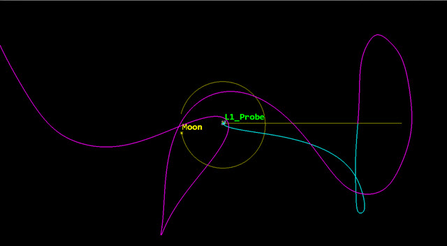
Third libration point maneuver
Without an orbital station-keeping strategy, the probe's trajectory departs from the L1 region after just one orbit.
Modeling orbital station-keeping at the L1 point
Add an orbital station-keeping strategy to maintain the libration point orbit over time using an Automatic Sequence.
Creating a new Automatic Sequence
The Automatic Sequence Browser contains a list of all Automatic Sequences defined for an Astrogator satellite. Each Automatic Sequence appears in the list with an identifying Name and User Comment field.
- Return to L1_Probe's () Properties ().
- Click Automatic Sequence Browser (
 ) in the MCS toolbar.
 - Click in the Automatic Sequence Browser dialog box.
- Enter Station Keeping in the Name field when the Field Editor dialog box opens.
- Click to accept your changes and to close the Field Editor dialog box.
Editing the Station Keeping Automatic Sequence
Add a station-keeping strategy using a Target Sequence to maintain the libration point orbit over time.
- Select Station Keeping in the Automatic Sequence Browser dialog box.
- Click .
- Click Insert Segment After (
 ) in the MCS toolbar when the Automatic Sequence Properties dialog box opens.
 - Select Target Sequence () in the Segment Selection dialog box.
- Click to accept your selection and to close the Segment Selection dialog box.
- Right-click on Target Sequence () in the MCS.
- Select Rename in the shortcut menu.
- Rename Target Sequence () Maintain LPO.
Inserting a Maneuver segment
Add a station-keeping Maneuver segment in the Maintain LPO Target Sequence.
- Click Insert Segment After () in the MCS toolbar.
- Select Maneuver () in the Segment selection dialog box.
- Click to accept your selection and to close the Segment selection dialog box.
- Nest Maneuver () in the Maintain LPO () Target Sequence.
- Click Segment Properties () in the MCS toolbar.
- Enter SK Burn in the Name field of the Edit Segment dialog box.
- Open the Color drop-down list.
- Select white.
- Click to accept your changes and to close the Edit Segment dialog box.
Setting the attitude
Set the X (Velocity) as a control parameter and use the custom Sun Syst_SEM_L1 axes as the attitude control.
- Select the Attitude tab.
- Open the Attitude Control drop-down list.
- Select Thrust Vector.
- Select the X (Velocity) target () to set it as the control parameter.
- Click the Thrust Axes ellipsis ().
- Select Sun () in the object tree when the Select Reference dialog box opens.
- Expand () Syst_Sem_L1 () in the Axes for: Sun list.
- Select Axes ().
- Click to accept your selection and to close the Select Reference dialog box.
Inserting a Propagate segment
Insert a Propagate segment after SK Burn.
- Click Insert After () in the MCS toolbar.
- Select Propagate () in the Segment Selection dialog box.
- Click to accept your selection and to close the Segment Selection dialog box.
- Click Segment Properties () in the MCS toolbar.
- Enter Prop to Plane Cross in the Name field when the Edit Segment dialog box opens.
- Open the Color drop-down list.
- Select a color that's different than all the other Propagate () segments in the scenario.
- Click to accept your changes and to close the Edit Segment dialog box.
Setting a stopping condition
Insert a Z-X Plane Cross stopping condition.
- Click New... () in the Stopping Conditions panel toolbar.
- Select Z-X Plane Cross () when the New Stopping Condition dialog box opens.
- Click to accept your selection and to close the New Stopping Condition dialog box.
- Select the Duration stopping condition.
- Click Delete () in the Stopping Conditions panel toolbar.
Updating Z-X Plane Cross's propagator
Use the Cislunar propagator to model the station-keeping orbit.
- Click the Propagator ellipsis ().
- Select Cislunar () in the Select Component dialog box.
- Click to accept your selection and to close the Select Component dialog box.
Setting the minimum propagation time and tolerance
You want to propagate the orbit for a total of 10 days.
- Click .
- Enter 864000 sec in the Minimum Propagation Time field when the Propagator Advanced dialog box opens.
- Click to accept your change and to close the Propagator Advanced dialog box.
- Enter 1e-06 km in the Tolerance field.
Updating Z-X Plane Cross's coordinate system
Use the SEM L1 coordinate system for the Propagate segment.
- Click the Coord. System ellipsis ().
- Select Sun () in the object tree of the Select Reference dialog box.
- Select Syst_SEM_L1 () in the Systems for: sun list.
- Click to accept your selection and to close the Select Reference dialog box.
Setting VxL1 as the result
You want the X component of the velocity needs to be nearly zero at the Rotating Libration Point (RLP) X-Z plane crossing. Use the VxL1 component as the result for the Propagate segment.
- Click .
- Expand () the Cartesian Elems () folder in the Available Components list when the User-Selected Results - Prop To Plane Cross dialog box opens.
- Select VxL1 ().
- Click Insert Component ().
- Click to accept your selection and to close the User-Selected Results - Prop To Plane Cross dialog box.
Adding a Return segment
Use a Return segment to control the execution of the Mission Control Sequence by returning control to its parent segment. If the MCS encounters an active Return segment, it will not run any segments after it in the MCS (or subsequence, if it belongs to one).
- Select SK Burn () in the MCS.
- Click Insert Segment After () in the MCS toolbar.
- Select return () when the Segment Selection dialog box opens.
- Click to accept your selection and to close the Segment Selection dialog box.
- Select the Enable (except Profiles bypass) option.
The return segment is active except when run from a Target Sequence profile (for example, a Differential Corrector), which will ignore it. When it converges, the SK Burn segment is executed again once (with the right Delta-V value) and the control is passed back to the main sequence.
Setting the Differential Corrector's control parameter
Update the control parameter's perturbation and maximum step (Max Step). Perturbation is the value that you want the profile to use in calculating numerical derivatives. Max Step is the maximum increment to the value of the parameter in a step.
- Select Maintain LPO () in the MCS.
- Click Properties... () in the Profiles panel toolbar.
- Select the Use check box for ImpulsiveMnvr.Pointing.Cartesian.X in the Control Parameters panel when the Differential Corrector dialog box opens.
- Set the following options:
| Option | Value |
|---|---|
| Perturbation | 0.05 m/sec |
| Max Step | 10 m/sec |
Setting the Equality Constraints (Results) parameters
Update VxL1's tolerance. The profile will stop when it achieves a value within this range of the Desired Value.
- Select the Use check box for VxL1 in the Equality Constraints (Results) panel.
- Enter 0.05 m/sec in the Tolerance field.
- Click to accept your changes and to close the Differential Corrector dialog box.
Setting the action to run active profiles
Set the Mission Control sequence to allow the active profiles to operate.
- Open the Action drop-down list.
- Select Run active profiles.
- Click to accept your changes and to close the Automatic Sequence Properties dialog box.
- Click to close the Automatic Sequence Browser dialog box.
- Click to accept your changes and to keep the Properties Browser open.
Using the automatic sequence
Apply the automatic sequence to the Z-X Plane Cross stopping condition.
- Select LPO () in the MCS.
- Select the On check box for Z-X Plane Cross in the Stopping Conditions panel.
- Click the Sequence ellipsis ().
- Select Station Keeping () when the Select Component dialog box opens.
- Click to accept your selection and to close the Select Component dialog box.
- Click to accept your changes and to keep the Properties Browser open.
Running the Mission Control Sequence
Rerun the entire Mission Control Sequence with the station-keeping Automatic Sequence enabled.
- Click Run Entire Mission Control Sequence () in the MCS toolbar.
- Click Clear Graphics () in the MCS toolbar.
- Click to accept your changes and to close the Properties Browser.
Viewing the changes in the 3D Graphics window
View the results of implementing the station-keeping Automatic Sequence.
- Bring the 3D Graphics window to the front.
- Use your mouse to set the view so that you can see the L1_Probe's () entire orbit.
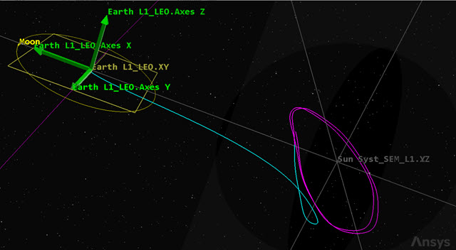
orbital station-keeping at L1
If you're going to perform further analysis, remember to reset all target sequences including the Automatic Sequence. A useful way to reset all active target sequence priorities at once is by clicking MCS Options (![]() ) in the MCS toolbar, selecting the Targeting tab in the MCS Options dialog box and clicking in the Active Profiles panel.
) in the MCS toolbar, selecting the Targeting tab in the MCS Options dialog box and clicking in the Active Profiles panel.
Creating a Maneuver Summary report
Now that you have modeled the probe's orbit and visualized its behavior, examine the results with a Maneuver Summary report that provides a summary of L1_Probe's maneuvers. The probe is propagated ahead in time by the LPO segment until it reaches the Duration condition (365 days) that stops the execution. In the meantime, each time there is a plane crossing, the Station Keeping Automatic Sequence is fired, bringing back the needed Delta-V for orbit maintenance.
- Right-click on L1_Probe () in the Object Browser.
- Select Report & Graph Manager... (
 ) in the shortcut menu.
 - Select the Maneuver Summary (
 ) report in the Installed Styles () folder in the Styles panel.
 - Click .
- Scroll through the Maneuver Summary report.
You can see that the first maneuver was the LEO Injection thrust. This burn had the largest estimated finite burn duration, Delta-V, and fuel used. This is because the probe is lifting off of Earth, which requires the most energy. Afterward, you can see the reported number of times the Station Keeping Automatic sequence was fired. By scrolling through the report you can review the estimated finite burn duration, Delta-V, and fuel used, which are all much smaller than the initial burn. The L1 point is unstable, and while you don't need as much fuel or Delta-V to maintain the probe's orbit for the specified mission time, it is still an important component to know when modeling a mission.
- Close the report and the Report & Graph Manager when finished.
Saving your work
Clean up your workspace and save your work.
- Close any open reports, properties and tools.
- Save () your work.
Summary
This scenario showed you how to configure your 2D and 3D Graphics windows for space operations and situational awareness. You learned how to create multiple assembled systems using the Vector Geometry tool. You created a custom Cartesian calculation component using the Component Browser. Using all the custom components you created, you made best guesses to inject a Satellite object modeling a probe in a libration point orbit around the Sun-Earth libration point, L1. Using a control parameter, your Satellite object came very close to establishing an orbit. Finally, you created an Automatic Sequence which enabled you to use station-keeping maneuvers to keep the probe in orbit around the L1 point.