Bounding Sphere |
While under development, the Insight3D development team wrote a series of blog posts, which are now archived here to provide in-depth technical information about some of the underlying techniques and design decisions. These posts reflect the work-in-progress state of the product at the time.
The following blog post was originally published on the Insight3D blog on February 5, 2008 by Deron Ohlarik. At the time of publishing, Insight3D was referred to by its development code-name, "Point Break".
The first maxim of improving frame rate is: the fastest way to draw an object is not to draw it. This has always been tempered with "unless determining not to draw it takes longer than drawing it." Ideally, for example, the triangles of a 3D model would not be sent to the GPU if the model were not visible. To check if each triangle of the model was visible or not would be too CPU intensive and result in a lower frame rate than always sending the model to the GPU.
Graphics applications typically create bounding spheres that encompass logical sets of triangles, such as a model. A sphere can quickly be checked for visibility. The model is drawn only if the bounding sphere is visible. Because the sphere doesn't exactly represent the 3D model, sometimes the model will be sent to the GPU even though the model isn't visible. Tighter bounding spheres reduce these false positives.
STK has always calculated bounding spheres for 3D models, terrain, et al. For Point Break, we decided to revisit our bounding spheres to see if we could calculate tighter spheres.
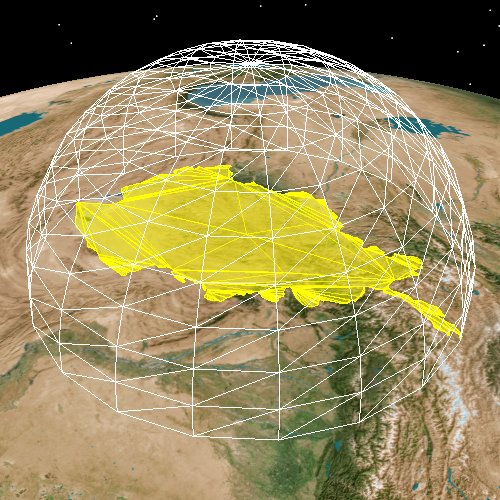
While I could find many bounding sphere algorithms on the web, I couldn't find timing and quality comparisons between these algorithms; so, I compared three popular algorithms myself using various area targets. If you are not familiar with STK area targets, they are areas on the Earth defined by a list of points that define the border and are filled inside, e.g., Afghanistan pictured above. STK calculates a bounding sphere from those points. All of the tested algorithms run in linear time, but vary in CPU usage.
The first algorithm is the simplest and fastest. I'll call it Naive. It is also the one we have always used in STK. In the first pass of the point data, an axis aligned bounding box is calculated, and the center of the sphere is the center of the box. In the second pass, the radius of the sphere is calculated as the point most distant from the center. This sphere and the time required to calculate the sphere is the baseline from which I compared the other algorithms. The drawback to this approach is that it almost never calculates the tightest sphere.
The second algorithm is Jack Ritter's and is documented in GRAPHICS GEMS I. The code can be downloaded here; the file is BoundSphere.c. A general description can be found here. Ritter's sphere is calculated in two passes like the Naive sphere. The first pass calculates an initial guess of the sphere. In the second pass, a point is added to the sphere one at a time. If the point lies within the sphere, nothing is done. If the point lies outside the sphere, the center and radius are modified to include the point. This is different from Naive that only modifies the radius.
This was the most frustrating of the algorithms. According to the author, the sphere is within 5% of the exact sphere, and isn't much slower to calculate than Naive. In my tests, there were spheres 19% worse than the Naive sphere much less the best, and there were spheres 11% better. This algorithm is highly dependent on the initial sphere and the order in which the points are added. I experimented with the initial sphere calculation. Adding just a few more compares to the code, I created an initial sphere that was larger than previously created. This change created a tighter sphere in many cases. For example, the sphere that was previously 19% worse than the Naive sphere was now the same. I suspect that if the initial sphere was based on the two points farthest from each other, the final sphere would typically be tighter than the original algorithm. I never tried that as calculating those two points would compromise the algorithm's speed.
The last algorithm I tried was Welzl's, which calculates the exact or minimum bounding sphere. The algorithm is based on the simple idea that the minimum bounding sphere is defined from two, three, or four of the points. All other points either lie on or within the sphere.
A significant shortcoming of this algorithm is that it takes a long time to compute relative to others. This isn't an issue if the sphere is calculated offline, but is if it is calculated in real-time. I tried both Bernd Gärtner's and Dave Eberly's implementations.
Here are the results of the different algorithms for five area targets:
Method | Time (msec) | Radius (m) | Time / Naive Time |
|---|---|---|---|
Naive | 0.009 | 296870 | 1.0 |
Ritter | 0.012 | 278722 | 1.3 |
Gärtner | 0.134 | 266354 | 14.8 |
Eberly | 0.185 | 266354 | 20.3 |
Method | Time (msec) | Radius (m) | Time / Naive Time |
|---|---|---|---|
Naive | 0.009 | 388544 | 1.0 |
Ritter | 0.012 | 350717 | 1.4 |
Gärtner | 0.151 | 348700 | 17.5 |
Eberly | 0.165 | 348700 | 19.3 |
Method | Time (msec) | Radius (m) | Time / Naive Time |
|---|---|---|---|
Naive | 0.020 | 648404 | 1.0 |
Ritter | 0.025 | 647093 | 1.2 |
Gärtner | 0.460 | 647093 | 23.3 |
Eberly | 0.282 | 647093 | 14.3 |
Method | Time (msec) | Radius (m) | Time / Naive Time |
|---|---|---|---|
Naive | 0.032 | 1229436 | 1.0 |
Ritter | 0.041 | 1286992 | 1.3 |
Gärtner | 0.930 | 1206456 | 28.9 |
Eberly | 0.605 | 1206456 | 18.8 |
Method | Time (msec) | Radius (m) | Time / Naive Time |
|---|---|---|---|
Naive | 0.479 | 3802142 | 1.0 |
Ritter | 0.581 | 3715345 | 1.2 |
Gärtner | 33.625 | 3711390 | 70.2 |
Eberly | 10.562 | 3711390 | 22.0 |
Welzl's exact solution was 11% better for the first two and nearly the same for the remaining area targets.
Eberly and Gärtner calculated the same and smallest radius as is expected for Welzl's algorithm. While Eberly ran about 20 times slower than Naive, Gärtner ran more slowly as the number of points increased. Welzl is supposed to scale linearly to the number of points, so the Gärtner results were unexpected. Gärtner ran faster than Eberly for the lower number of points.
For the third area target, Ritter calculated the same radius as Welzl. Ritter also calculated a larger radius than Naive for the fourth area target, which isn't good since it took longer to run.
What does all this mean? We learned that using Naive in STK all these years hasn't been a catastrophe. We can improve our numbers, though.
I decided not to use Welzl because the improvement over Naive didn't justify additional time required to calculate the sphere.
Ritter takes only 20% more time than Naive and generally creates smaller spheres. However, Ritter sometimes creates larger spheres. Based on that, I decided to use a hybrid method as the default bounding sphere code for Point Break; Ritter and Naive are run simultaneously, and the code returns the smaller of the two spheres. This method increased the run time over Ritter only slightly. We can still run Naive and Ritter independently if needed. We expect to use Naive for objects that are constantly changing size or are short lived.