Horizon Culling 2 |
While under development, the Insight3D development team wrote a series of blog posts, which are now archived here to provide in-depth technical information about some of the underlying techniques and design decisions. These posts reflect the work-in-progress state of the product at the time.
The following blog post was originally published on the Insight3D blog on March 25, 2009 by Deron Ohlarik.
In a previous entry, I described a simple method for horizon culling. That method determined if one sphere, the occluder, occluded another sphere, the occludee, for example if a planet represented as a bounding sphere occluded a satellite represented as a bounding sphere. In this entry, I'll describe how to find if a planet occludes a part of itself. Normally, I write out all the math; however given my time constraints and in the interest of me finally writing another blog, I'll forego that.
3D GIS applications invariably render the Earth and other planets. A planet is generally organized as a hierarchy of terrain tiles of varying levels of detail. As the viewer moves closer and closer to particular part of a planet, higher and higher fidelity tiles are rendered. The Virtual Terrain Project has a nice list of terrain rendering algorithms. Frustum culling techniques are normally first applied to tiles, so that only tiles inside the view frustum are rendered. Next, horizon culling is applied.
We'll first look at the simplest case where the tile lies exactly on the occluder. In this example, the Earth is the occluder. The Earth is not a sphere, but an oblate spheroid. We must be conservative to ensure that tiles are not culled that are actually visible. To this end, the sphere that represents the Earth is the largest sphere still inside the oblate spheroid. The tile is the occludee. In contrast to the occluder to be conservative, the sphere must completely bound the tile.
In Figure 1, the planet is in yellow, the tile is in blue, and the tile bounding sphere is in light blue. If the viewer is anywhere in the dark green area defined by the two lines tangent to both the planet and the tile bounding sphere, the tile bounding sphere is not visible, and the tile is culled; anywhere else, the tile bounding sphere is visible, and the tile is rendered. Done. This is no different than that described in my first horizon culling entry.
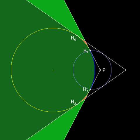
H0 and H1 are points on the planet of lines that are tangent to both the planet and tile bounding sphere. P is the center of the proxy bounding sphere of radius zero.
The tile bounding sphere is visible before the tile is actually visible. The tile is considered visible at H0 and H3, while ideally it should be visible at H1 and H2, the limits of the tile. If the horizon culling algorithm were more accurate, the tile would also be culled if the viewer were in the light green area. Woe!
A tighter bounding sphere can be computed, so tight in fact that the bounding sphere has a radius of zero. Lines H1P and H2P are tangent to the planet that intersect at P.
P is our new bounding sphere, a bounding sphere that is a point that bounds nothing. If P is visible, the tile is visible; If P is not visible, the tile is not visible. P is a proxy bounding sphere for the tile. Now using the proxy, the tile is not visible not only in the dark green area, but also in the light green area.
All is calmerfect in our circular world with our surface conforming tiles.
Sadly, tiles rarely conform. Figure 2 recasts the blue tile as one with n altitudes, An. How is P computed? The lower P's altitude, the better. The answer must be conservative. Each altitude becomes visible at different viewing angles. I don't know if I have the perfect answer, but I have an answer.
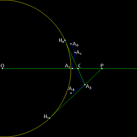
O is the center of the planet. C is the center of the tile bounding sphere. A0-4 are altitudes that define the tile. H0 and H1 are horizon points from the perspective of A3. P is the center of the proxy bounding sphere of radius zero.
The first step is to compute the bounding sphere of the tile in the typical way. We are only concerned with the center of the sphere, so some of the computations are not required. In Figure 2, C is the center. P will lie along OC, where O is the center of the planet.
Next, for each altitude determine the two lines that intersect the altitude and are tangent to the planet. For clarity of the figure, I show the lines only for A3, which are H0A3 and H1A3. Each line intersects OC. Of all the intersections, the intersection furthest from O will be P. In this case, A3 results in the furthest P, and that is along H1A3. Of course, the altitude associated with P will not always be the first visible depending on the direction that the viewer approaches the tile, but it yields the most conservative answer.
I've described the algorithm in terms of 2D, but it is simple enough to convert to 3D. It's just one more D. I could have described the algorithm in 1D. How would that have been for you?
Given particular arrangements of altitudes, P could become infinite or lie on the line not in the direction of OC; that is invalid. In those cases, I fall back to the traditional bounding sphere method.
I earlier mentioned that the method might not yield the lowest altitude P. I wrote that P must be along OC. I know that there are arrangements of altitudes where a different choice of C than the center of tile bounding sphere results in a lower P.
For our product, Insight3D, the proxy bounding sphere results in more tiles being culled over the traditional bounding sphere that would encompass a tile.
This method could also be applied to quickly cull cities, which share similar characteristics to and are often similarly tiled like terrain. If a city tile is determined to be visible, additional culling algorithms may be employed.