STK Pro, STK Premium (Air), STK Premium (Space), or STK Enterprise
You can obtain the necessary licenses for this tutorial by contacting AGI Support at support@agi.com or 1-800-924-7244.
The results of the tutorial may vary depending on the user settings and data enabled (online operations, terrain server, dynamic Earth data, etc.). It is acceptable to have different results.
The following tutorial introduces the Volumetric object and various spatial components from Analysis Workbench that model the volume of space covered by a spinning sensor subject to various geometric constraints.
Capabilities Covered
This lesson covers the following STK Capabilities:
- Analysis Workbench
- Coverage
- Volumetric Analysis
Problem Statement
Engineers and operators require a quick way to create calculations and conditions that depend on locations in 3D space which are, in turn, provided by user-definable volume grids. The grids can provide both analysis and general situational awareness. In this tutorial, you need to determine the following in a 3D volume of space:
- Distance and location from a ground site.
- Sensor visability.
- Accumulated sensor visibility against a moving target.
Solution
Use the Spatial Analysis tool to create calculations and conditions that depend on locations in a user-defined 3D grid. Combine the spatial calculations and volume grids in the Volumetric object to report and graph calculations over time and across grid points. Then, visually depict the volume representing various values interpolated across the grid points.
Upon completion of this tutorial, you will be able to create the following:
- Simple cartographic grids.
- Constrained grids.
- Spherical grids on moving objects.
- Spatial calculations.
Creating the STK Scenario
The Volumetric Analysis tutorial requires a basic knowledge of how to use STK, including creating and populating a scenario, setting up 3D visualization, and animating a scenario. If you are a new STK user, follow Beginner tutorials to learn the basics of STK before attempting to perform the steps in this tutorial.
The Volumetric Analysis tutorial is built on an STK scenario that contains a facility with a spinning sensor, an aircraft, and an area target. To create the scenario:
- Launch STK (
 ).
). -
Click the Create a Scenario (
 ) button.
 - Enter the following in the STK: New Scenario Wizard:
- When you finish, click .
| Option | Value |
|---|---|
| Name: | VolumetricTutorial |
| Stop: | + 90 sec |
Adding a Sensor
-
Using the Insert STK Objects Tool (
 ) insert a
Facility (
) insert a
Facility ( ) using the Insert Default method.
 - Insert a Sensor (
 ) using the Define Properties (
 ) method.
 - Select Facility1 as its parent object.
- Open Sensor1's properties.
- On the Basic - Definition page, set Cone Half Angle to 15 deg.
- On the Basic - Pointing page, change the Pointing Type to Spinning.
- Change the Spin Rate to 10 revs/min.
- Change the Spin Axis Elevation to 50 deg.
- Leave Azimuth at 0 deg and Cone Angle at 20 deg.
- Click to apply the changes.
Adding an Area Target
- Insert an Area Target (
 ) using the Define Properties () method.
 - On the Basic - Boundary page, make the following changes:
- Area Type: Ellipse.
- Semi-Major Axis: 7 km
- Semi-Minor Axis: 4 km
- Bearing: 45 deg
- On the Basic - Centroid page, make the following changes:
- Latitude: 40.0386 deg
- Longitude -75.5966 deg
- On the Constraints - Basic page, select Minimum Elevation and set it to 90 deg, which will constrain visibility to everything within the area target.
- Click .
- Insert an Aircraft (
 ) using the Define Properties () method.
- On the Basic - Route page, insert the following three points:
- Click .
- Open VolumetricTutorial's properties ().
- On the Basic - Time page, under Animation:
- Select the Stop at Time check box.
- Set the step size to 0.5 sec.
- Click .
- Save the scenario.
| Latitude | Longitude | Altitude | Turn Radius |
|---|---|---|---|
| 39.9966 deg | -75.6391 deg | 3.668 km | 1.6858 km |
| 40.0929 deg | -75.6204 deg | 3.668 km | 1.6858 km |
| 40.1253 deg | -75.5595 deg | 3.668 km | 1.6858 km |
Using the Spatial Analysis Tool and Creating a Volumetric Object
The Spatial Analysis tool allows you to create calculations and conditions that depend on locations in 3D space which are, in turn, provided by user-definable volume grids. Combining spatial calculations and volume grids in volumetric objects enables you to report and graph calculations over time and across grid points, as well as visually depict volumes representing various values interpolated across grid points.
Using the Spatial Analysis Tool
The following steps show how to use the Spatial Analysis tool to create a Simple Cartographic Grid.
- Right-click AreaTarget1 () and select Zoom To to center the 3D Graphics window on the object.
- Close the 2D Graphics window and the Timeline View.
- Right-click AreaTarget1 in the Object Browser and select Analysis Workbench… (
 ).
). - Select the Spatial Analysis tab. The Spatial Analysis tab is used to create the following spatial components:
- Spatial Calculation (
 ), which is a scalar calculation that depends on both time and location.
- Spatial Condition (
 ), which is a condition that depends on both time and location.
- Volume Grid (
 ), which is a collection of enumerated points placed in 3D space using steps taken in each coordinate using various coordinate types.
- Click to create a new Volume Grid and set the following parameters:
- Type: Cartographic
- Name: SimpleCartographic
- Clear the Constrain active grid points within Area Target check box.
- Click
 .
. - Set the following parameters in the Altitude section:
- Minimum: 0 km (default)
- Maximum: 10 km
- Number of Steps: 20
- Click twice to apply the changes and create the new grid. The SimpleCartographic grid is added under My Components.
- Select Aircraft1 in the left pane of Analysis Workbench.
-
Click to create a new Volume Grid and set the following parameters:
- Type: Spherical
- Name: SimpleSphere
- Click .
- Set the following parameters:
- Click twice to apply the changes and create the new grid. The SimpleSphere grid is added under My Components.
- Click to dismiss the Analysis Workbench.
| Field Name | Azimuth | Elevation | Range |
|---|---|---|---|
| Minimum | 0 deg | -90 deg | 0.5 km |
| Maximum | 360 deg | 90 deg | 1 km |
| Number of Steps | 36 | 18 | 1 |
Creating a Volumetric Object
The Volumetric object is defined in terms of components from the Analysis Workbench. It also enables you to define various graphics properties, and has associated data providers for reporting and graphing.
- Open the Insert drop down and select Default Object... .
- Select Volumetric (
 ), then click .
 - Open Volumetric1's properties.
- On the Basic - Definition page, click
 next to Volume Grid to bring up the Volume Grid selector from Analysis Workbench.
 - Select AreaTarget1 on the left and SimpleCartographic on the right.
- Click to assign the selected volume grid to Volumetric1.
- Click and view the grid in the 3D Graphics window.
- On the Volumetric1 Basic - Definition page, select the Spatial Calculation check box, then click to access the Spatial Calculation selector from Analysis Workbench.
- Select Aircraft1 on the left and the Distance on the right, and click .
- Click to assign all selections to Volumetric1.
Analysis Workbench displays the STK objects on the left and the Spatial Analysis components on the right.
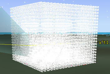
In the 3D Graphics Window, notice that the SimpleCartographic grid is now visible in the 3D Graphics window. This illustrates the extent of space covered by the grid as well as granularity of the grid.
Compute Volumetric Data
- Right-click Volumetric1 in the Object Browser and expand the Volumetric menu.
- Select Compute to initiate evaluation of volumetric data over time and across the grid.
- Go to the Volumetric1 3D Graphics - Volume page and notice that this color corresponds to active grid points. All active grid points are included when evaluating volumetric data. This may not always be the case, which is discussed in subsequent exercises.
- Switch from Active Grid Points to Spatial Calculation Levels.
- Under Show Fill Levels, click
 and set the following values:
 - Start Value: 0
- Stop Value: 16
- Step: 4
- Click .
- Go to the Volumetric1 3D Graphics - Legends page and select the Show Legend check box on the Fill Legend tab.
- Make the following changes:
- Change the Title to Aircraft1 Straight Line Distance (km).
- Set the Color Square Width (pixels) to 50.
- Click .
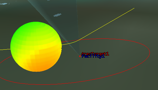
- Go to the 3D Graphics window and notice that concentric circles of different colors appear on the outside of the grid. Zoom in and out and rotate the view to observe how colors appear on the outside from different directions and how they change on the inside. These colors represent a straight line distance from Aircraft1.
- Animate the scenario and notice how the straight line distance graphics for the aircraft change over time.
Once the computation is completed, the entire grid volume will be filled with the color specified on the Volumetric1 3D Graphics - Volume page.
Double-click on a few points to get the exact value. Close the grid point information window.
Change the Spatial Calculations
- Go to the Volumetric1 Basic - Definition page.
- Click Spatial Calculation to again bring up the spatial calculation selector from Analysis Workbench.
- Select Facility1 on the left and Altitude on the right.
- Click to assign selected spatial calculations to Volumetric1.
- Click to assign all selections to the volumetric object. Re-evaluation of new volumetric data over time and across the grid is initiated and the Progress indicator is displayed.
- Go to the Volumetric1 3D Graphics - Legends page and change the Title to Facility1 Altitude (km).
- Click to dismiss the Volumetric1 properties.
- In the 3D Graphics window, observe its behavior again.
- Save the scenario.
The grid volume is filled with horizontal layers of colors, each representing a different vertical distance value.

Using a Spatial Calculation based on Condition Satisfaction
In addition to directly limiting which grid points are considered for volumetric computations, spatial conditions can also produce calculations based on their satisfaction intervals. This can be accomplished by using a type of Spatial Calculation called Spatial Condition Satisfaction Metrics.
- Right-click Sensor1 in the Object Browser and select Analysis Workbench… ().
- Select the Spatial Analysis tab.
- Click to create a new Spatial Calculation and define the following parameters:
- Type: Spatial Condition Satisfaction Metrics
- Name: AccumulatedVisibilityDuration
- Click Spatial Condition to bring up the Spatial Condition selector from Analysis Workbench.
- Select Facility1 - Sensor1 on the left and Visibility on the right.
- Click to assign the selection and return to the Add Spatial Analysis Component page.
- Set the following on the Add Spatial Analysis Component page:
- Satisfaction Metric: Interval Duration
- Duration Type: Sum (default)
- Accumulation Type: Up To Current Time
- Filter: None (default)
- Click to apply your changes and create the spatial condition.
- Click to dismiss the Analysis Workbench.
Reset the Volumetric Data
- Double-click Volumetric1 and on the Volumetric1 3D Graphics - Volume page, select Spatial Calculation Levels.
- Highlight all previously selected values, then click .
- On the Basic - Definition page, click Volume Grid to bring up Volume Grid selector from the Analysis Workbench.
- Select AreaTarget1 and the SimpleCartographic volume grid.
- Click to assign the selected volume grid to Volumetric1.
- On the Basic - Definition page, click Spatial Calculation to bring up Spatial Calculation selector from Analysis Workbench.
- Select Facility1 - Sensor1 on the left and AccumulatedVisibilityDuration on the right.
- Click to assign selected volume to volumetric object.
- Click to assign all selections to the volumetric object. Re-evaluation of new volumetric data over time and across the grid will be initiated. The Progress indicator may appear.
- If you don't have the Volumetric set to auto-compute when changes are made, you should right-click on the Volumetric object in the Object Browser and select Volumetric > Compute.
Set the New Volumetric Values
- Go to the Volumetric1 3D Graphics - Volume page and click and set the following values:
- Start Value: 0
- Stop Value: 30
- Step: 3
- Click .
- Select the Display colors outside min/max check box.
- Go to the 3D Graphics - Legends page and clear the Show Legend check box.
- Click .
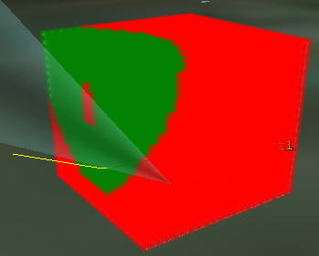
- Go to the 3D Graphics window. Animate and observe how changing colors reflect accumulated visibility duration at different grid points as spinning sensors sweeps through them.
- On the Volumetric1 3D Graphics - Volume page, make the color associated with the zero (0) sec level completely translucent to better observe internal structure of the volume being swept as durations are being accumulated during animation.
- Change the translucency of other levels to better observe other parts of the volume being swept.
- On the Volumetric1 3D Graphics - Grid page, clear the Show Grid check box to better observe the volumetric display.
- Click to apply all changes and dismiss the page.
- Save the scenario.
![]()

Using a Constrained Grid
A constrained grid provides an opportunity to dynamically restrict analysis to within certain time and spatial limits as dictated by a selected spatial condition, while still retaining the regular lattice structure of the underlying grid.
- Right-click AreaTarget1 in the Object browser and select Analysis Workbench… ().
- Select the Spatial Analysis tab.
- Click to create a new Volume Grid and set the following:
- Type: Constrained
- Name: SimpleCartographicInFOV
- Click Reference Grid to bring up Volume grid selector from Analysis Workbench.
- Select AreaTarget1 on the left and SimpleCartographic on the right.
- Click to assign the selection.
- Click Spatial Condition to bring up the Spatial Condition selector from Analysis Workbench.
- Select Facility1-Sensor1 on the left and Visibility on the right.
- Click to assign the selection
- Click to apply your changes and create the new grid.
- Click to dismiss Analysis Workbench.
Set the New Volumetric Values
- On Volumetric1 Basic - Definition page, click Volume Grid to bring up Volume grid selector from Analysis Workbench.
- Select AreaTarget1 on the left and SimpleCartographicInFOV on the right.
- Click to assign the selected volume grid to Volumetric1.
- Click to accept the new grid and recalculate.
- On the Basic - Interval page, keep the default At Instant in time option selected for an evaluation of the spatial calculation.
- On the Volumetric1 3D Graphics - Grid page, select the Show Grid check box to better observe the volumetric display.
- Click to assign all selections to the Volumetric1.
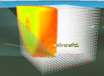
- The volume covered by these active grid points can be displayed separately from any calculation. To do that, open the Volumetric1 3D Graphics - Volume page and select the Active Grid Points option. The multi-color display representing levels of spatial calculation are replaced with a single color corresponding to active grid points. Animate and observe how this volume follows the sensor FOV.
- Right-click Volumetric1 and select Report & Graph Manager... (
 ).
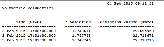
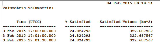
). - Double-click the Satisfaction Volume report style. The report will look similar to the following:
- Save the report as a quick report (
 ), and then close the report.
 - Save the scenario.
The volumetric display restricts all colors to within the sensor Field of View (FOV) because only grid points that appear inside the sensor FOV are active and are used to evaluate and display volumetric data.


Using Spatial Conditions for a Constrained Grid
You can create new spatial conditions using various operations provided in Analysis Workbench. Any of these user-defined conditions can be used to constrain a grid.
- Right-click Sensor1 in the Object browser and select Analysis Workbench… ().
- Select the Spatial Analysis tab.
- Click to create a new Spatial Condition and set the following:
- Type: Over Time
- Name: VisibilityOverTime
- Click Original Spatial Condition to bring up Spatial Condition selector from Analysis Workbench.
- Select Facility1 - Sensor1 on the left and Visibility on the right.
- Click Reference Intervals to bring up the Time Interval and Interval List selector from Analysis Workbench.
- Select Facility1 - Sensor1 on the left and AvailabilityTimeSpan on the right.
- Click .
- Click again to create the new spatial condition.
Notice that Duration Type is set to Static.
Add a New Volume Grid
- Select AreaTarget1 and click to create a new Volume Grid and make the following selections:
- Type: Constrained
- Name: SimpleCartographicInFOR
- Click Reference Grid to bring up Volume grid selector from Analysis Workbench.
- Select AreaTarget1 on the left and SimpleCartographic on the right.
- Click to assign the selection.
- Click Spatial Condition to bring up the Spatial Condition selector from Analysis Workbench.
- Select Facility1 - Sensor1 on the left and VisibilityOverTime on the right.
- Click to assign the selection.
- Click to apply the page and create the new grid
- Click to dismiss Analysis Workbench.
- Double-click Volumetric1 object and on the Volumetric1 Basic - Definition page, click Volume Grid to bring up Volume grid selector from Analysis Workbench.
- Select AreaTarget1 on the left and select SimpleCartographicInFOR on the right.
- Click to assign the selected volume grid to volumetric object.
- Click to assign new selection to the volumetric object.
- On the 3D Graphics - Volume page, select the Spatial Calculation Levels option, and observe that horizontal color slices now appear with the sensor FOR.
- Click to apply all changes and close the page.
- Refresh the SatisfactionVolume report or recreate it from the Quick Report Manager to display the accumulated coverage.
- Save the scenario.
Re-evaluation of new volumetric data over time and across the grid will be initiated. Progress indicator may appear.
New volumetric display restricts all colors to within the sensor FOR, which covers space to which sensor has visibility over specified period of time.
Using a Geographically Constrained Grid
You can define Line and Area Target objects in STK and then use them to define spatial conditions that geographically restrict volume grids.
- Notice that AreaTarget1 covers an elliptical shape under the volume grid.
- Right-click AreaTarget1 in the Object browser and select Analysis Workbench… ().
- Select the Spatial Analysis tab.
- Right-click SimpleCartographic under My Components and select Properties...
- Select the Constrain active grid points within Area Target check box.
- Click to apply the changes.
- Right-click Volumetric1 in the Object Browser and select Volumetric > Compute.
- On Volumetric1 3D Graphics - Grid page, clear the Show Grid check box to better observe the constrained colored volume.
- Save the scenario.
The Volumetric display and computations will be cleared.
Re-evaluation of new volumetric data over time and across the grid is initiated and the Progress indicator is displayed.
The new volumetric display restricts all colors to within an elliptical cylinder limited by the elliptical shape of AreaTarget1.
Using a Grid Attached to a Moving Object
You can define volumetric objects using volume grids attached to moving objects.
- Clear the check box next to Volumetric1 in the Object Browser to turn off Volumetric1 object graphics to avoid cluttering the display.
- Open the Insert drop down and select Default Object... .
- Select Volumetric (), then click .
- Open Volumetric2's properties.
- On the Basic - Definition page, click next to Volume Grid to bring up the Volume Grid selector from Analysis Workbench.
- Select Aircraft1 on the left and the SimpleSphere on the right.
- Click to assign the selected volume grid to the volumetric object.
- Select the Spatial Calculation check box, and click to access the Spatial Calculation selector from Analysis Workbench.
- Select Facility1 - Sensor1 on the left and the AccumulatedVisibilityDuration on the right.
- Click to assign the selected spatial calculation to Volumetric2.
- Click to assign the new selection to Volumetric2.
- Right-click the Volumetric2 object and select Volumetric > Compute.
- Go to the 3D Graphics - Volume page, switch to Spatial Calculation Levels, click , and set the following values:
- Start Value: 0
- Stop Value: 15
- Step: 3
- Click .
- Go to the 3D Graphics - Grid page and clear the Show Grid check box for a better display.
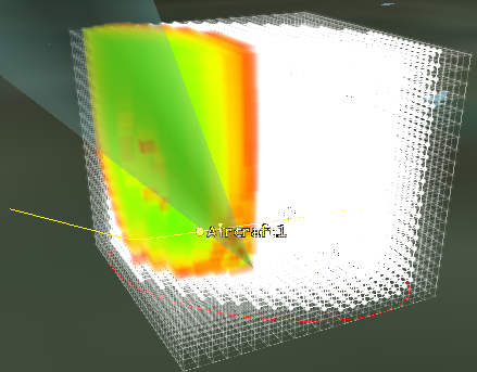
- Animate and observe how accumulated Sensor1 visibility to grid points surrounding Aircraft1 evolves over time.
Evaluation of new volumetric data over time and across the grid is initiated and the Progress indicator is displayed.