STK Premium (Space) or STK Enterprise
You can obtain the necessary licenses for this tutorial by contacting AGI Support at support@agi.com or 1-800-924-7244.
Required product install: The Ansys ModelCenter® model-based systems engineering software and the STK Plugin for ModelCenter are required to complete this tutorial.
ModelCenter installation prerequisites: The ModelCenter software requires the installation of a 64-bit version of Java, a 64-bit implementation of Python 3.x, and the installation of the thrift and six Python packages. See the ModelCenter Installation Prerequisites for more information.
This tutorial was written using version 2026 R1 of the Ansys ModelCenter® model-based systems engineering software.
The results of the tutorial may vary depending on the user settings and data enabled (online operations, terrain server, dynamic Earth data, etc.). It is acceptable to have different results.
Capabilities covered
This lesson covers the following capabilities of the Ansys Systems Tool Kit® (STK®) digital mission engineering software:
- STK Pro
- Astrogator
- STK Analyzer
Problem statement
Engineers and mission planners want to know what effects small launch errors can have on a mission. You have a nominal trajectory for a launch, which you planned using the STK/Astrogator® capability, but you want to better understand how small uncertainties can compound over time, should the launch not go exactly as planned.
Solution
Use the STK/Astrogator® capability and the Analyzer capability, which is part of the Ansys ModelCenter® model-based systems engineering software, to vary the burnout latitude, longitude, altitude, and velocity, then look at the resulting changes in a satellite's Keplerian elements.
Using the starter scenario
To speed things up and allow you to focus on the portion of this exercise that teaches you how to use the ModelCenter software, a partially created scenario has been provided for you.
Opening the starter scenario
The starter scenario is included in your install.
- Launch the STK application (
 ).
). - Click
 Open a Scenario in the Welcome to STK dialog box.
 - Browse to <Install Dir>\Data\Resources\stktraining\VDFs.
- Select Analyzer_LaunchErrors.vdf.
- Click .
Saving the VDF as a scenario file
Save and extract the VDF data in the form of a scenario folder. When you save a VDF in the STK application, it will save in its originating format. That is, if you open a VDF, the default save format will be a VDF (.vdf). If you want to save and extract a VDF as a scenario folder, you must change the file format by using the Save As feature. This will create a permanent scenario file complete with child objects and any additional files packaged with the VDF.
- Open the File menu when the starter scenario opens.
- Select Save As....
- Select the STK User folder in the navigation pane when the Save As dialog box opens.
- Select the Analyzer_LaunchErrors folder.
- Click .
- Select Scenario Files (*.sc) in the Save as type drop-down list.
- Select the Analyzer_LaunchErrors scenario file in the file browser.
- Click .
- Click in the Confirm Save As Dialog box to overwrite the existing scenario file in the folder and to save your scenario.
A scenario folder with the same name as the VDF was created for you when you opened the VDF in the STK application. This folder contains the temporarily unpacked files from the VDF.
When saving a VDF as a scenario folder, you should extract its contents to the scenario folder the STK application automatically creates for you in the STK User folder. See the
Save (![]() ) often during this lesson!
) often during this lesson!
Reviewing the starter scenario
Take a moment to familiarize yourself with the starter scenario.
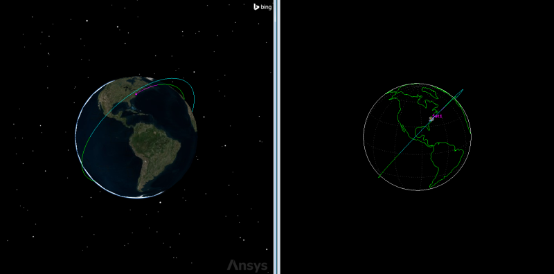
Launch Errors 3D and 2D Graphics windows
Viewing the satellite's initial state
Review the Launch parameters of the Astrogator satellite by viewing its Mission Control Sequence. The
- Right-click on Sat1 (
 ) in the Object Browser.
 - Select Properties (
 ).
). - Select WallopsLaunch (
 ) in the Mission Control Sequence.
 - Ensure the Launch tab is selected.
- Review the Launch parameters.
- Select the Burnout tab.
The WallopsLaunch
Take note of the launch coordinates. Your launch is taking place from Launch Complex 0 of the Mid-Atlantic Regional Spaceport on Wallops Island, Virginia.
Note the time of flight, altitude, and other burnout parameters. You will vary these values as part of your trade studies.
Reviewing the initial Propagate segment
The satellite is moved to its ascending node using a Propagate segment, which models the movement of the spacecraft along a trajectory until meeting specified stopping conditions.
- Select PropToAscendingNode (
 ) in the MCS.
 - Note the Stopping Condition.
Understanding the RaiseApogee Target Sequence
The satellite's apoapsis (apogee) is raised using a Target Sequence. A
- Select Mnvr1 (
 ) in the MCS.
 - Select ToApogee () in the MCS.
- At the bottom of the MCS, click .
- Close (
 ) the User-Selected Results dialog box without making any changes.
Note that Mnvr1 is an Impulsive ![]() ) to make it an independent variable as part of the target sequence.
) to make it an independent variable as part of the target sequence.
Note the Apoapsis stopping condition.
Clicking this button opens the User-Selected Results dialog box, in which you can view and select calculation objects for Astrogator to report and target when defining a Differential Corrector Target Sequence profile. In this case, you are targeting the true altitude above Earth.
Viewing the RaiseApogee differential corrector
The Target sequence uses a
- Select RaiseApogee (
 ) in the MCS.
 - Click Properties... () in the Profiles toolbar.
- Review the targeting profile's properties when the Differential Corrector dialog box opens.
- Close () the Differential Corrector dialog box without making any changes.
Looking at the Variables, the control parameter is Cartesian.X — or X (Velocity) — which was targeted. The equality constraint is altitude and the desired value is set to 2000 kilometers.
Understanding the RaisePerigee Target Sequence
After satellite's apogee is raised as part of the RaiseApogee Target Sequence, its periapsis is raised using another Target Sequence, RaisePerigee.
- Select Impulsive Maneuver () in the MCS.
- At the bottom of the MCS, click .
- Close () the User-Selected Results dialog box without making any changes.
Note that Both X (Velocity) and Y (Normal) are selected (![]() ), making them independent variables in the Target Sequence.
), making them independent variables in the Target Sequence.
Note that both Eccentricity and Inclination are the selected results.
Viewing the RaisePerigee differential corrector
A Differential Corrector Profile runs the Target Sequence.
- Select RaisePerigee () in the MCS.
- Click Properties... () in the Profiles toolbar.
- Close the Differential Corrector dialog box.
- Click to Close the Properties Browser without making any changes.
Looking at the variables, the control parameters are Cartesian.X and Cartesian.Y — or Y (Normal) — which were targeted. The equality constraints are eccentricity and inclination. The desired eccentricity value is 0 and inclination is 50 degrees.
Creating a new ModelCenter project
The
- Save (
 ) your scenario.
 - Close the STK application.
- Open the ModelCenter (
 ) application.
 - Click in the Welcome to ModelCenter dialog box.
- Click when the What type of model would you like to create? dialog box opens.
- Navigate to your scenario folder (for example, C:\Users\<username>\Documents\STK_ODTK 13\Analyzer_LaunchErrors.
- Enter Analyzer_LaunchErrors in the File name field.
- Ensure the Save as type is set to the ModelCenter Model (Zip) (*.pxcz).
- Click .
Launching the STK Plugin for ModelCenter
The
- Select favorites (
 ) in the Server Browser at the bottom of the window.
 - Click and drag the STK component (
 ) into the dashed circle underneath "Drop items here to build the model" in the workflow's Analysis View.
 - Select Analyzer_LaunchErrors.sc when the Open STK Scenario file dialog box opens.
- Click .
- After a few moments, the STK Analyzer window will open.
The Analyzer_LaunchErrors scenario file will open in the STK application in the background.
You can add any of the STK variables as ModelCenter input or output variables through the STK Analyzer window that appears. If you change the value of a variable in your scenario through the STK interface or the ModelCenter Component Tree, you should re-add the variable into ModelCenter or re-run the workflow before running any trade studies with the new value.
Setting up your analysis with Analyzer
Use the STK Analyzer window to configure the input and output variables available for further analysis with the
Selecting the Analyzer input variable
Your studies will focus on the Trip value (that is, the true anomaly) of the first propagate segment against the Delta-V of the maneuver segment. Select the Trip value as your input variable.
- Select Sat1 () in the STK Variables tree.
- Expand (
 ) the Propagator (Astrogator) (
 ) property in the STK Property Variables tree.
 - Select WallopsLaunch ().
- Select BurnoutVelocity_FixedVelocity (
 ).
). - Move (
 ) BurnoutVelocity_FixedVelocity () into the Analyzer Variables list.
 - Move () the following input variables to the Analyzer Variables list:
- Burnout_Geodetic_Latitude
- Burnout_Geodetic_Longitude
- Burnout_Geodetic_Altitude
When you select an object in the STK Variables tree, all possible input variable candidates for that object are listed under the General tab and the Active Constraints tab in the STK Property Variables panel.
Be sure you do not select the Launch_Geodetic Latitude, Longitude, and Altitude variables.
Note that all of the variables are listed under Inputs in the Analyzer Variables list.
Selecting the Analyzer output variables
You want to analyze the effects of the launch errors on the final propagated orbit. Add the orbital parameters from the final Propagate segment in the MCS as your output variables.
- Expand () Prop10Mins ().
- Expand () the FinalState () property.
- Expand () the Keplerian () property.
- Select SemiMajorAxis (
 ).
). - Move () SemiMajorAxis () into the Analyzer Variables list.
- Move () the following output variables () to the Analyzer Variables list:
- Eccentricity
- Inclination
- RAAN
- ArgOfPeriapsis
- TrueAnomaly
- Click to confirm your selections and to close the STK Analyzer window.
Note that these variables are listed under Outputs in the Analyzer Variables list.
This will also close the STK application, which had been running in the background.
Studying launch errors with probabilistic analysis
You want to better understand how uncertainties during the launch can affect your intended orbit. Use the Probabilistic Analysis tool to run a trade study of the burnout parameters against the final orbital parameters.
Opening the Probabilistic Analysis tool
The Probabilistic Analysis tool helps you understand how uncertainties in the design parameters affect the outputs of the ModelCenter model. The tool is typically used to compute the probability that the value of an output variable exceeds a specified limit. In addition to random sampling methods such as the Monte Carlo method, the tool provides a number of additional analytical methods that require much smaller sample sizes. You can set up and execute the probabilistic analysis through a unified graphical user interface (GUI). Using the GUI, you can easily switch between available algorithms.
- Expand (
 ) all the elements in the Component Tree.
 - Click Probabilistics (
 ) in the Standard toolbar.
Selecting the design variables and responses
It is important to properly specify the distribution characteristics of the design variables. When a new design variable is added to the tool, the Distribution Selection dialog box will appear. Using the Select dialog box, you can choose a distribution for a given design variable
- Click and drag BurnoutVelocity_FixedVelocity (
 ) to the Design Variables field.
 - Select Normal (
 ) in the Distribution list when then Select Distribution dialog box appears.
 - Leave the default Mean setting as is.
- Change the Std. Dev setting to 0.001%.
- Click to confirm your changes and to close the Select Distribution dialog box.
- Using the above process, click and drag Burnout_Geodetic_Latitude (), Burnout_Geodetic_Longitude (), and Burnout_Geodetic_Altitude () to the Design Variables field, leaving their Mean settings at their default values and setting their standard deviations (Std. Dev.) to 0.001%.
- Multi-select all six of the Keplerian element output variables (
 ) — SemiMajorAxis, Eccentricity, Inclination, RAAN, ArgOfPeriapsis, and TrueAnomaly.
 - Click and drag the variables to the Responses field.
The Normal distribution type is a "bell-shaped" distribution that describes many situations where observations are distributed symmetrically around the mean. For this distribution, 68% of all values under the curve lie within one standard deviation of the mean, and 95% lie within two standard deviations.
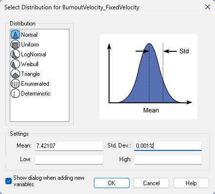
Distribution selection dialog box
Running the probabilistic analysis
With your input and output variables added, set up and run your probabilistic analysis.
- Leave Monte Carlo as the Method.
- Change the Number of Runs to 100.
- Click .
Monte Carlo is a random sampling technique. It generates random values for the design variables based on the joint distribution of the design variables. The samples are then evaluated for computing response variable values. Since this is a random sampling technique, if ModelCenter performs a high enough number of evaluations, this method will give the most accurate results. The number of evaluations to generate a good probability estimate increases rapidly as the probability value under consideration decreases. Since Monte Carlo is a random sampling technique, you can use it with response functions, discrete design variables, and discrete response variables that are not smooth. The histogram plot ignores failed runs while calculating mean, variance, skewness, kurtosis, etc.
This control parameter is the maximum number of runs the tool will perform.
Clicking will open the Data Explorer, which is a tool used by Trade Study tools to display data while they are being collected from your Model. While data are being collected, the Data Explorer displays a progress meter, a halt button, and the data. The Table page of the Data Explorer displays trade study data in a tabular form. It is the default window that is present for all trade studies. Cells are shaded differently depending on the associated variable's state. Input variables are shown with green text, valid values are displayed with black text, invalid values are displayed with gray text, and modified values are displayed with blue text. From the table it is possible to view and edit all values in your trade study and even to add and remove whole runs.
Viewing the Histogram Plot
Once the trade study is complete and all data have been collected, the Data Explorer toolbar becomes active. The Data Explorer stores values for all variables in a workflow and special variables from the trade study. Some trade study tools will automatically launch a default plot window when the trade study runs. For other plots, you can create them from the Add View menu.
In this case, a Histogram Plot is automatically created. A Histogram Plot visualizes the distribution of a variable in a trade study. In addition to a graphical Histogram representation of the data, the page also contains a Box Plot of the distribution as well as a display of the statistics of the distribution, including mean, standard deviation, quantiles, etc. Finally, the Histogram page contains bounds on which values of the variable are acceptable and computes reliability statistics based on how many runs fall into that defined space.
- Review the Histogram Plot.
- Click Dimensions in the Plot Options menu on the left-hand side of the Histogram Plot.
- Open the x drop-down list.
- Select Eccentricity.
- Click on the plot to close the Plot Options menu.
- Review the results.
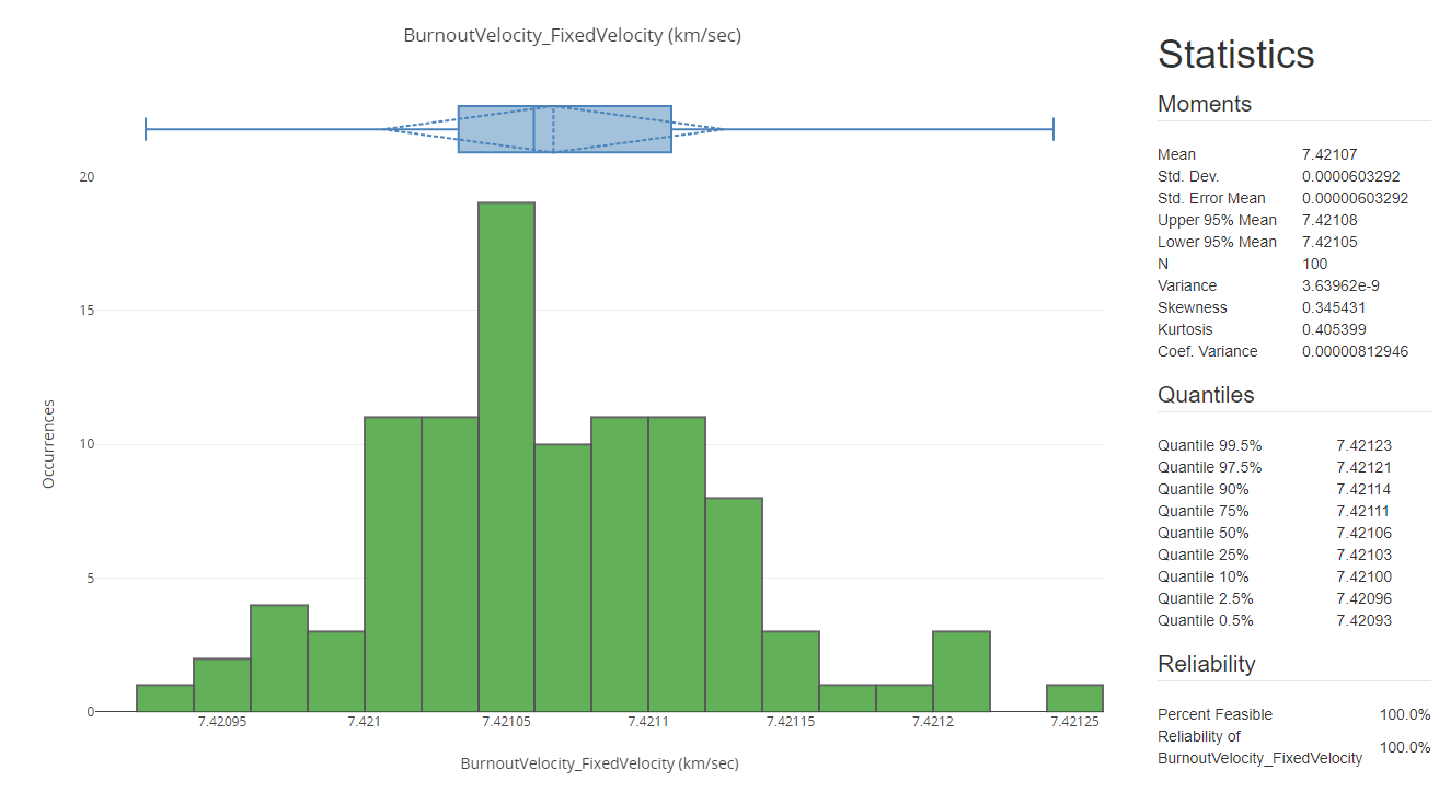
Burnout Velocity Histogram Plot
In this case, the Histogram Plot shows data for the first variable in the Design Variables field, the Burnout Velocity.
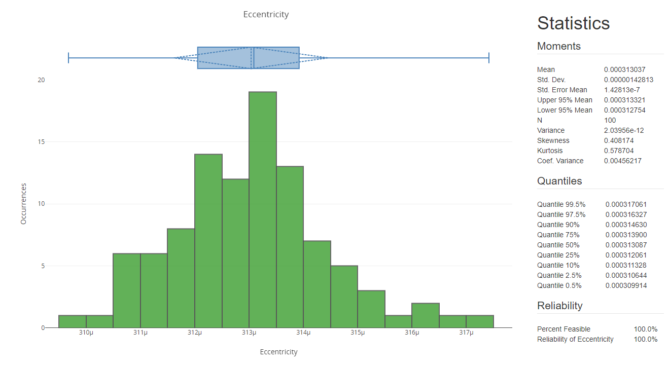
Eccentricity Histogram Plot
You can cycle through each of the Keplerian elements in this manner.
Generating a Scatter Matrix
A Scatter Matrix displays a grid of graphs that compare every design variable and response against every other design variable and response in the trade study. It is a grid of 2D scatter plots, where all variables under investigation are plotted against each other. Scatter matrices are an effective way to visualize trends and all possible two-way interactions of the data.
- Click Add View (
 ) on the Histogram Plot toolbar.
 - Select Scatter Matrix (
 ) in the drop-down menu.
 - Review the scatter plots.
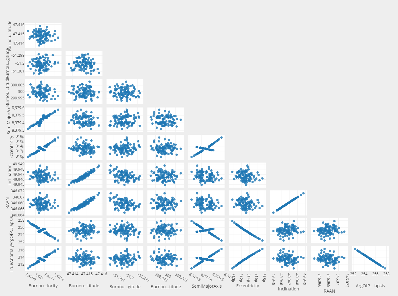
Scatter Matrix Plot
Using these scatter plots, it's possible to gain an understanding as to the relationship between various variables in the trade study.
Creating a Variable Importance Summary Plot
A Variable Importance plot allows you to see which individual design parameters (main effects) and combinations of design parameters (interaction effects) have the most influence on the currently selected output variable. This plot helps you to quickly zero in on the most important design parameters for your problem.
- Click Add View () on the Scatter Matrix toolbar.
- Select Variable Importance Summary Plot (
 ) in the drop-down menu.
 - Review the plots.
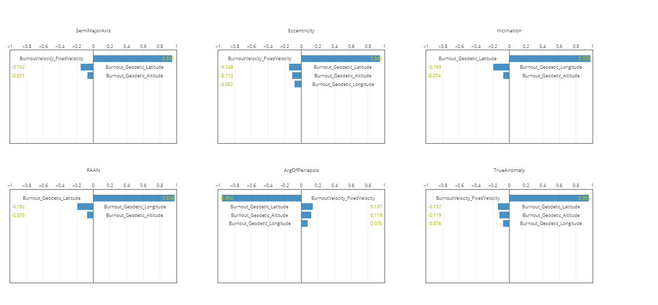
Variable Importance Summary Plot
From the plots, it is clear that the burnout velocity and burnout latitude have the greatest effects on the satellite's orbital state. Using this information, you can choose which launch parameters to study in greater depth.
Saving your work
Save your work and close out ModelCenter application.
- Close out any open plots, tools, and the Data Explorer window.
- Click when prompted to close your trade study without saving.
- Click Save (
 ) to save your ModelCenter workflow.
 - Close the ModelCenter application.
Summary
You began by opening a prebuilt scenario with a satellite propagated from launch using the Astrogator capability. After examining the satellite's burnout parameters, you used the ModelCenter software to better understand how uncertainties in the launch can affect the mission design by conducting a probabilistic analysis. By using the ModelCenter software, you can better understand your design space and plan accordingly.
On your own
While you can use ModelCenter to better understand how launch errors can affect your mission and inform ts design, it does not help you correct for errors once the satellite has been launched. For that, you can use the Ansys Orbit Determination Tool Kit (ODTK®) orbital measurement processing software and the STK software together to plan and model maneuvers needed to get your mission back on track. See the Using Astrogator and ODTK Together tutorial for more information.