STK Premium (Space) or STK Enterprise
You can obtain the necessary licenses for this tutorial by contacting AGI Support at support@agi.com or 1-800-924-7244.
ModelCenter installation prerequisites: The ModelCenter software installs the current version of Java and Python supported by Ansys, but you can also use your own versions. See the Installation instructions in the ModelCenter Installation Guide and Supported Versions documentation for more information. Contact AGI support for help with installation.
This tutorial was written using version 2026 R1 of the Ansys ModelCenter® model-based systems engineering software. Refer to the ModelCenter Supported Versions page in the ModelCenter Installation Guide and Supported Versions documentation for compatibility information.
The results of the tutorial may vary depending on the user settings and data enabled (online operations, terrain server, dynamic Earth data, etc.). It is acceptable to have different results.
Capabilities covered
This lesson covers the following capabilities of the Ansys Systems Tool Kit® (STK®) digital mission engineering software:
- STK Pro
- Coverage
- STK Analyzer
- STK SatPro
Problem statement
Engineers and operators require a quick way to determine how various mission components can be changed and the impact of doing so on the overall effectiveness of the mission. You want to design and test a new satellite constellation to provide persistent stereo coverage over a ground site. You have a defined orbital regime in which you must remain, but you can vary the number of satellites you launch.
Solution
Use the SatPro capability and a Satellite Collection object to model your satellite constellation together with the Coverage tool, part of the Coverage capability, to model coverage over a single site. Then, use the Analyzer capability, which is part of the ModelCenter model-based systems engineering software, and the Design of Experiments (DOE) tool to vary the number of orbital planes and the satellites therein to identify the configuration that best meets your requirements.
What you will learn
Upon completion of this tutorial, you will understand the following:
- How to use the Coverage tool to model single-object coverage
- How to use a Satellite Collection object and single-object coverage with the ModelCenter application
- How to define and perform a design of experiments with the ModelCenter application
Creating a new scenario
First, you must create a new scenario, and then build from there.
- Launch the STK application (
 ).
). - Click
 Create a Scenario in the Welcome to STK dialog box.
 - Enter the following in the STK: New Scenario Wizard:
- Click when you finish.
- Click Save (
 ) when the scenario loads.
 - Verify the scenario name and location in the Save As dialog box.
- Click .
| Option | Value |
|---|---|
| Name | Analyzer_DOE |
| Location | Default |
| Start | Default |
| Stop | Default |
The STK application creates a folder with the same name as your scenario for you.
Save () often during this scenario!
Disabling streaming terrain
By default, the STK application connects to the Ansys Geospatial Data Cloud to distribute Earth terrain data for analysis and visualization. Turn off
- Right-click on Analyzer_DOE () in the Object Browser.
- Select Properties (
 ) in the shortcut menu.
 - Select the Basic - Terrain page when the Properties Browser opens.
- Clear the Use terrain server for analysis check box in the Terrain Server panel.
- Click to confirm your change and to close the Properties Browser.
Modeling a constellation with a Satellite Collection object and the Walker tool
A
Creating the seed satellite
The
- Bring the Insert STK Objects tool (
 ) to the front.
 - Select Satellite (
 ) in the Select An Object To Be Inserted list.
 - Select Define Properties () in the Select A Method list.
- Click .
Propagating a Satellite object using properties
You can propagate a Satellite object using the
- Select the Basic - Orbit page when the Property Browser opens.
- Enter the following orbital parameters:
- Keep the remaining default parameters.
- Click to confirm your changes, propagate the Satellite object, and to close the Properties Browser.
- Right-click on Satellite1 () in the Object Browser.
- Select Rename in the shortcut menu.
- Rename Satellite1 () Seed_Sat.
| Option | Value |
|---|---|
| Semimajor Axis | 7158 km |
| Inclination | 45 deg |
Creating a new Satellite Collection object
Insert a new Satellite Collection object into your scenario using the Walker Tool method.
- Bring the Insert STK Objects tool () to the front.
- Insert a Satellite Collection object (
 ) using the Walker Tool () method.
Using the Walker tool
Use the Walker tool to
- Click Seed Satellite: when the Walker tool opens.
- Select Seed_Sat () when the Select Object dialog box opens.
- Click to confirm your selection and to close the Select Object dialog box.
- Leave the Pattern Type set to Delta in the Shell properties panel.
- Set the following parameters for the satellite collection:
- Enter Walker_Collection in the Name field in the Container Options panel.
- Click to propagate the Walker_Collection Satellite Collection object.
- Click to close the Walker tool.
- Clear the check box for Seed_Sat () in the Object Browser.
In a Delta pattern, the orbit planes are evenly distributed over 360 degrees around the central body.
| Option | Value |
|---|---|
| Number of Sats per Plane | 1 |
| Number of Planes | 1 |
| Inter Plane Phase Increment | 0 |
You do not need to visualize the seed satellite for this analysis.
Inserting the ground site
Your ground site is located in Boulder, Colorado, in the United States. Model it by inserting a
- Bring the Insert STK Objects tool () to the front.
- Insert a Place (
 ) object using the From City Database (
 ) method.
 - Enter Boulder in the Name field when the Search Standard Object Data dialog box opens.
- Click .
- Select Boulder - Colorado in the Results list.
- Click .
- Click to close the Search Standard Object Data dialog box.
Defining single-object coverage
Your mission is to create a constellation with persistent stereo coverage over a single ground site. To evaluate the quality of coverage over a single object in the STK application, you can use the Coverage tool to define
Opening the Coverage tool
Your coverage analysis will focus on your ground site. Open the Coverage tool with Boulder.
- Right-click on Boulder () in the Object Browser.
- Select Coverage... (
 ) in the shortcut menu.
Selecting the assets an computing coverage
A
- Select the AllSatellites (
 ) satellite subset in the Assets list when the Coverage Tool opens.
 - Click .
- Leave the grouping set to Separate.
- Click .
When assigning a Constellation, Satellite Collection, or a Chain object containing constellations as an Coverage asset, you can characterize all the objects in the Constellation, or Satellite Collection object as a single asset (Grouped) or as separate assets (Separate). See Using Grouped Assets for more information.
Computing coverage in the STK application's Coverage tool is necessary to use single-object coverage with the ModelCenter application.
Defining the quality of coverage
You can evaluate the quality of coverage for an object by choosing the method for computing coverage, setting measurement options, and identifying the criterion needed to achieve satisfactory coverage. By default, all single-object coverages are defined with a Simple Coverage Figure Of Merit type; change it to the N Asset Coverage type. The
- Click in the Figure of Merit panel.
- Open the Type drop-down list in the Definition panel when the Specify Figure of Merit dialog box opens.
- Select N Asset Coverage.
- Open the Compute drop-down list.
- Select Minimum.
- Click to confirm your selections and to close the Specify Figure of Merit dialog box.
- Note the Value of the Figure Of Merit, beneath the FOM type.
- Select the Save Configuration check box.
- Click to confirm your changes and to close the Coverage tool.
This will compute the minimum number of assets available over the entire coverage interval. The value is an integer, which is useful if the coverage definition contains a large number of assets.
When the STK application computes coverage for the object, it also computes the static value for the Figure Of Merit type you chose. The minimum number of assets available over the entire coverage interval value is 0, since you only have one satellite in your collection and it does not have access at all times.
This tells the STK application to save the single-object coverage definitions when the scenario is saved to disk, assuming that you already computed coverage.
It's important to select this check box when using single-object coverage for analysis with the ModelCenter application, otherwise the STK application won't save the coverage data and your ModelCenter project will not work.
Saving your STK scenario
Before opening the ModelCenter application, save your scenario to save the accesses you computed and close out of the STK application.
- Save () your scenario.
- Close the STK application.
Creating a new ModelCenter project
The Ansys ModelCenter model-based systems engineering software is designed for multidisciplinary analysis and design optimization. It allows you to automate complex workflows, integrate multiple engineering tools, and optimize designs within model-based systems engineering (MBSE) frameworks. By wrapping tools and analysis programs like the STK application and running them in an automated fashion, the ModelCenter software makes the design process more efficient, saves engineering time, and reduces the chances for error in the design process. It implements MBSE processes flexibly; its drag-and-drop graphical user interface can be used to assemble tools into a complete engineering workflow, which can contain branches, loops, logical statements, and more. Your workflow can contain tools that run on any number of different machines and operating systems. Once a repeatable engineering analysis process is created, you can repeatedly execute the process, using parallel computing resources if available. Each execution corresponds to a different set of inputs, which you can use to explore and quantify the performance of your design alternatives in a relatively short time.
- Open the ModelCenter (
 ) application.
 - Click in the Welcome to ModelCenter dialog box.
- Click when the What type of model would you like to create? dialog box opens.
- Navigate to your scenario folder (for example, C:\Users\<username>\Documents\STK_ODTK 13\Analyzer_DOE).
- Enter Analyzer_DOE in the File name field.
- Ensure the Save as type is set to the ModelCenter Model (Zip) (*.pxcz).
- Click .
A Process is a graphical, flowchart-like workflow that explicitly tells the ModelCenter application what order (and under what conditions) to run each component.
You can learn more about the ModelCenter software
Launching the STK Plugin for ModelCenter
All ModelCenter workflows are built using a simple drag-and-drop scheme for creating a graphical layout of a complex analysis. Process workflows leverage that capability by highlighting "hot spots" for adding and moving components in a workflow. Components encapsulate an analysis or control function. Each component exposes input and output variables and executes a run method to transform inputs into outputs. The
- Select favorites (
 ) in the Server Browser at the bottom of the ModelCenter window.
 - Click and drag the STK component (
 ) into the hot spot — the dashed circle — underneath "Drop items here to build the model" in the workflow's Analysis View.
 - Select Analyzer_DOE.sc when the Open STK Scenario file dialog box opens.
- Click .
This will open the STK scenario and STK Analyzer windows. Please be patient.
The Analyzer_DOE scenario file will open in the STK application in the background. If the STK application opens in front of the ModelCenter application, bring the ModelCenter application window back to the front.
Setting up your analysis with Analyzer
Use the STK Analyzer window to configure the input and output variables available for further analysis with the
Selecting the Analyzer input variables
You need to select both input and output variables from the main Analyzer window. Start by adding the input variables, which, in this case, are the two variables about your constellation you can change — the number of planes and the number of satellites per plane.
- Select Walker_Collection () in the STK Variables tree.
- Expand (
 ) the Walker (
 ) property.
 - Expand () the Shell1 () property.
- Select the Planes (
 ) input variable.
 - Move (
 ) the Planes () input variable to the Analyzer Variables list.
 - Select the SatellitesInPlanes () input variable.
- Move () the SatellitesInPlanes () input variable to the Analyzer Variables list.
- Note both variables are listed under Inputs in the Analyzer Variables list.
When you select an object in the STK Variables tree, all possible input variable candidates for that object are listed under the General tab and the Active Constraints tab in the STK Property Variables panel.
You can also move variables to the Analyzer Variable list by double-clicking on a variable.
Defining the output variables
Now that the input variables are defined, you can add the output variables. In this case, you want to use the
- Select Boulder () in the STK Variables tree.
- Select the Object Coverage () tab in the Data Provider Variables panel.
- Expand () the FOM Static Value data provider (
 ).
). - Select the FOM Static Value (
 ) data provider element.
 - Move () the FOM Static Value () data provider element to the Analyzer Variables list.
- Note that the Values (
 ) output variable is listed under Outputs in the Analyzer Variables list.
 - Click to confirm your selections and to close the STK Analyzer window.
- Note that the Analysis View now contains an STK_ODTK13 () component, which is shown as a box in the Analysis View window.
This will also close the STK application, which had been running in the background.
Running your model
The ModelCenter Component Tree, on the left side of the ModelCenter window, shows a hierarchical view of your workflow. It lists each component and its variables, lets you view or edit values, and gives a quick view of the variable state, including invalid input and output variables. Expanding a component shows its variables. In this case, you must open all the components to expose the input and output variables and run your model before performing a design of experiments.
- Expand (
 ) all the components in the Component Tree.
 - Note the variable values in the Component Tree.
- Click Run (
 ) on the Standard toolbar.
 - When completed, note that Values[0]'s name has been updated to Values[1] and its icon has changed from invalid (
 ) to valid (
 ).
). - Expand () Values[1] ().
- Note that a child, Values[0], is now present after running your model, and it has a Value of 0.
- Double-click on Values[1] () to open the Large Data Monitor.
- Close the Large Data Monitor without making any changes when finished.
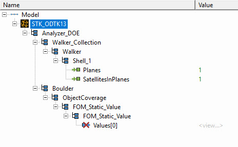
expanded component tree
These are the values imported into the ModelCenter application from the Analyzer_DOE scenario. Input variables, like Planes ( ), you can change. Output variables, like Values[0] (), are calculated and supplied by the component based on the input variables. In this case , the brackets ([ ]) indicate that Values[0] () is a long array variable. Values[0] () is invalid, meaning that it has not yet been calculated. The ModelCenter application keeps track at all times of which variables are valid and which are invalid.
This is the minimum number of assets available over the entire coverage interval, which you previously noted in the Coverage tool.
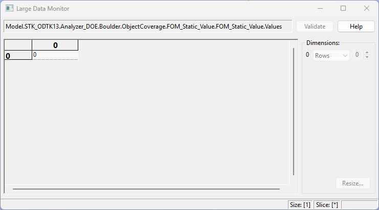
Large Data Monitor
The Large Data Monitor is used to view and edit data that are too large to view in the component tree or as a convenient view for arrays. For arrays like Values[1] (), the Large Data Monitor shows 2D slices of the array, allowing for the easy viewing and editing of elements. At the bottom of the Large Data Monitor is the status of the array's size, as well as which slice is currently being viewed. In this case, in spite of the data type being a long array, your array is very small — just 1 by 1.
Using the Design of Experiments tool
The ModelCenter software features a suite of trade study tools to help you create and analyze your workflows. A trade study is a structured exploration of a workflow by running many designs and collecting the resulting data. Trade studies systematically vary inputs and record responses, allowing you to understand a design space, compare alternatives, and identify optimal or robust designs. Once a workflow is built, these exploration tools can drive it without knowing how the results are computed; essentially, they treat a workflow as a black box, repeatedly getting and setting variables until an objective is met or a plan of experiments is complete. Trade study results can then used to visualize and understand significant trends and trade-offs.
The Design of Experiments (DOE) tool simplifies purposeful changing of inputs (design variables) in a workflow to observe the corresponding changes in outputs (response variables). A set of valid values for constitutes a design point. This tool is sued to collect the responses in the workflow to a set of predetermined design points. You can use the Design of Experiments tool to create and perform tables of predetermined runs for a scenario. You can either use a classical design type, such as a Full Factorial design, or supply your own custom table of runs.
Opening the Design of Experiments tool and adding the design variables
Use the Design of Experiments tool to find out how many satellites and planes you need to provide persistent two-satellite coverage over the ground site.
- Click DOETool (
 ) on the Standard toolbar.
 - Click and drag the Planes () input variable from the Component Tree to the Design Variables field when the Design of Experiments tool opens.
- Open the drop-down list (
 ) in the Values field.
 - Select Low: High: Levels: .
- Click and drag the SatellitesInPlanes () input variable from the Component Tree to the Design Variables field.
- Open the drop-down list () in the Values field.
- Select Low: High: Levels: .
Adding bounds to the design variables
For each design variable, you must set the values for the upper and lower bounds as well as the number of steps to take between those values.
- Click on the blank line after each property and enter the following values:
- Note that there are now 140 runs in the Design panel.
| Name | Low | High | Levels |
|---|---|---|---|
| Model.STK_ODTK13.Analyzer_DOE.Walker_Collection.Walker.Shell_Walker_Group.Planes | 2 | 11 | 10 |
| Model.STK_ODTK13.Analyzer_DOE.Walker_Collection.Walker.Shell_Walker_Group.SatellitesInPlanes | 2 | 15 | 14 |
This gives you a large variety of satellite and plane combinations to run through. The number you place in the Levels field equate to the number of runs you want to complete. To obtain data from a combination of both design variables based on their Low and High settings will take a total of 140 runs (10 × 14).
Selecting the response variable and running the design of experiments
Critical response variables are the factors of the model about which you are trying to gain an understanding. To perform your design of experiments, you must specify a response variable.
- Click and drag Values[0] from the Component Tree to the Response Variables field.
- Click to execute your design of experiments and to open the Data Explorer.
Since your are completing 140 runs, this will take some time. Please be patient.
Clicking will open the Data Explorer, which is a tool used by Trade Study tools to display data while they are being collected from your Model. While data are being collected, the Data Explorer displays a progress meter, a halt button, and the data. When you run a design of experiments, it will first build a table of runs. These runs consist of all combinations of the two design variables for their specified ranges and number of steps. After the table has been created, it will run through each case and store values in the Data Explorer.
Viewing the results
Once the trade study is complete and all data have been collected, the Data Explorer toolbar becomes active. The Data Explorer stores values for all variables in a workflow and special variables from the trade study. Some trade study tools will automatically launch a default plot window when the trade study runs. For other plots, you can create them from the Add View menu. For this study, create a 3D Scatter Plot to better understand your results. A 3D Scatter Plot displays an X-Y plot of variables in the workflow.
- Bring the Data Explorer to the front when the when the DOE test is finished running.
- Click Add View (
 ) on the Data Explorer toolbar.
 - Select 3D Scatter Plot (
 ) in the drop-down menu.
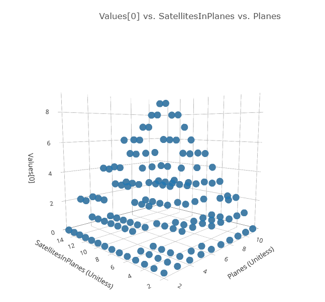
3D scatter plot
Constraining the figure of merit value
The Figure of Merit value you are interested in is the minimum number of satellites that have access to the ground site. For this mission, at least two satellites need to have concurrent access at all times for the mission to be considered successful. Add constraints to the plot to specify the upper and lower limits on your figure of merit value.
- Click Constraints (
 ) in the plot options menu.
 - Click Uncheck All (
 ) on the Values[0] line to clear all the values from the Values[0] variable when the Constraints dialog box opens.
 - Select the check box for 2 for Values[0].
- Click anywhere on the 3D Scatter Plot to confirm your changes and to close the Constraints menu.
- Examine the 3D Scatter Plot.
- Hover your cursor over one of the design points (the blue dots) to display a Design Tooltip.
- Close the 3D Scatter Plot when you are finished.
By default, the figure of merit value entries are individually enumerated with a check box next to each value. While you can click Switch to Continuous Mode ( ) to turn enumerated values into a slider to filter out undesirable designs, for this study, keep the values enumerated.
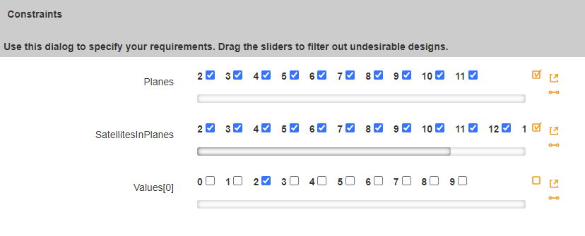
enumerated constraints
In this case, your limits are a single enumerated value — 2.
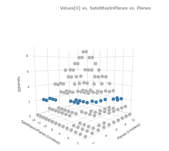
Updated 3D scatter plot
The plot displays the feasible results in blue. The infeasible results you are not interested in are retained, but grayed out.
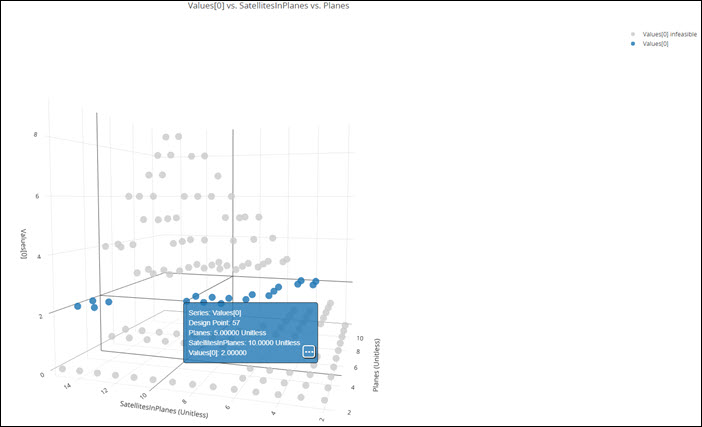
3D Scatter plot with Design Tooltip
In the above view, in order to get a minimum of two satellites accessing Boulder at any given time, it'll take ten satellites in five orbital planes for a total of 50 satellites. However, if you hover over other design points, the combinations are different.
Using the Data Explorer
You can use the Data Explorer to search for your values to determine which combination gives you the fewest number of accesses that provide continuous coverage utilizing the fewest number of satellites.
- Bring the Data Explorer to the front.
- Right-click on response(Model.STK_ODTK13.Analyzer_DOE.Boulder.ObjectCoverage.FOM_Static_Value.FOM_Static_Value.Values[0]) in the AUTO SCROLL list.
- Select Sort Runs in the shortcut menu.
- Select Ascending in the Sort Runs submenu.
- Scroll until you find a combination where you have a FOM value of 2 and the fewest number of satellites (SatellitesInPlanes × Planes).
- Close the Data Explorer.
- Click when prompted to close your trade study without saving.
- Close the Design of Experiments tool.

Sorted Runs
You may have multiple combinations that work. For example, you could have 10 orbital planes with 4 satellites in each plane, or 5 orbital planes with 8 satellites per plane. Choose the combination that best fits your requirements.
This will also close all open plots and graphs.
Saving your work
Save your work and close out ModelCenter application.
- Click Save (
 ) to save your ModelCenter workflow.
 - Close the ModelCenter application.
Updating the values in your STK scenario
While you can't update your STK scenario directly from the ModelCenter application, you can use the values you found and update it in the STK application yourself by reopening your scenario and making the necessary changes.
Reopening the Analyzer_DOE scenario
Open the Analyzer_DOE scenario and update Walker_Collection's parameters.
- Launch the STK application ().
- Click
 Open a Scenario in the Welcome to STK dialog box.
 - Browse to your scenario folder (for example, C:\Users\<username>\Documents\STK_ODTK 13\Analyzer_DOE).
- Select Analyzer_DOE.sc.
- Click .
Updating Walker_Collection's properties
Apply the changes to Walker_Collection.
- Open Walker_Collection's () Properties ().
- Select the Basic - Definition page when the Properties Browser opens.
- Select the Shells - Name - 1 row in the Walker Properties panel.
- Click Edit selected shell (
 ) on the Shells toolbar.
 - Enter the value you determined for Planes (for example, 5) in the Planes field when the Edit Shell dialog box opens.
- Enter the value you determined for SatellitesInPlanes (for example, 8) in the Satellite in Planes (Slots) field.
- Click to confirm your changes and to close the Edit Shell dialog box.
- Click to confirm your changes and to close the Properties Browser.
Reviewing the Figure Of Merit
Review the changes to your Figure Of Merit in the Coverage tool and generate an
- Right-click on Boulder () in the Object Browser.
- Select Coverage... () in the shortcut menu.
- Click in the Graphs panel when the Coverage tool opens.
- Review the FOM Value graph.
- Close the FOM Value Graph.
- Click to close the Coverage tool without making any changes.
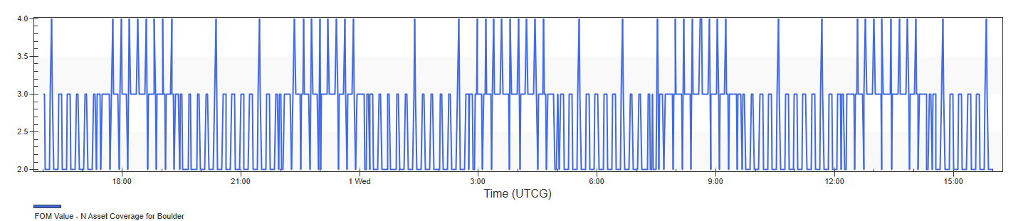
FOM Value Graph
Examining the orbital parameters for the satellites
An obvious question is how you determine where to place the satellites after launch based on the design of experiments you conducted. Generate an
- Right-click on Walker_Collection () in the Object Browser.
- Select Report & Graph Manager... (
 ) in the shortcut menu.
 - Select the All Satellites Walker (
 ) report style in the Installed Styles (
 ) list in the Styles panel when the Report & Graph Manager opens.
 - Click .
- View the data in the report.
- Close the All Satellites Walker report and the Report & Graph Manager when finished.
The report provides information about all 40 satellites in the satellite collection, including IDs, shells, planes, slots, and orbital elements.
Saving your work
Clean up your workspace and close out your scenario.
- Close any reports and tools you still have open.
- Save () your work.
Summary
You began by configuring a Walker satellite collection and computing single-object coverage over a ground site. Using the ModelCenter application's Design of Experiments tool, you selected a combination of satellites and planes utilizing a minimum number of satellites, a combination which met your mission requirement to provide persistent stereo coverage over the ground site. You then returned to the STK application and updated your scenario with the values you found from your design of experiments. Finally, you conducted additional analysis in the STK application with the values you determined.