STK Pro, STK Premium (Air), STK Premium (Space), or STK Enterprise
You can obtain the necessary licenses for this tutorial by contacting AGI Support at support@agi.com or 1-800-924-7244.
The results of the tutorial may vary depending on the user settings and data enabled (online operations, terrain server, dynamic Earth data, etc.). It is acceptable to have different results.
This tutorial requires STK 12.9 or newer to complete.
Capabilities covered
This lesson covers the following STK Capabilities:
- STK Pro
- Communications
- Coverage
Problem statement
Engineers and operators need to quickly determine high-frequency (HF) communication link budgets. Skywave propagation, sunlight / darkness at the site of transmission and reception, season, sunspots, and solar activity are some factors needed to be taken into consideration. In this lesson, you will perform three analyses in the following order:
- Analyze a near-vertical incidence skywave (NVIS)
- Analyze a long-distance communication link
- Analyze long-distance communications in a large coverage area
Solution
You will use STK Pro and STK's Communications and Coverage capabilities to model and analyze HF communications between two ground sites divided by mountainous terrain. You will model and analyze HF communications between two ground sites separated by thousands of kilometers. Finally, you will determine HF communication coverage over a large operations area for mission planning purposes.
What you will learn
Upon completion of this tutorial, you will understand the following:
- The VOACAP Radio Frequency Environmental model
- VOACAP data providers
- Dipole and external antenna patterns
In this tutorial, antenna design frequencies won't always match the actual transmission or received frequencies. Antenna lengths in this scenario simulate multiband antennas.
Video guidance
Watch the following video. Then follow the steps below, which incorporate the systems and missions you work on (sample inputs provided).
Creating a new scenario
Create a new scenario with an analysis period of 24 hours.
- Launch STK (
 ).
). - Click
 Create a Scenario in the Welcome to STK dialog box.
 - Enter the following in the STK: New Scenario Wizard:
- Click when finished.
- When the scenario loads, click Save (
 ). A folder with the same name as your scenario is created for you in the location specified above.
 - Verify the scenario name and location and click .
| Option | Value |
|---|---|
| Name | HF_Analysis |
| Location | Default |
| Start | 15 Apr 2024 19:00:00.000 UTCG |
| Stop | 16 Apr 2024 19:00:00.000 UTCG |
Save (![]() ) often!
) often!
Decluttering 3D Graphics window labels
Label Declutter is used to separate the labels on objects that are in close proximity for better identification in small areas.
- Bring the 3D Graphics window to the front.
- Click Properties (
 ) in the 3D Graphics window toolbar.
 - Select the Details page when the Properties Browser opens.
- Select the Enable check box in the Label Declutter panel.
- Click to accept the changes and close the Properties Browser.
Selecting the RF environment
A scenario's RF Environment properties enable you to model environmental factors that can affect the performance of a communications link. You can set them at the scenario level and also override or vary them at the individual STK object level.
- Right-click HF_Analysis () in the Object Browser.
- Select Properties () in the shortcut menu.
- Select the RF - Environment page when the Properties Browser opens.
Understanding VOACAP
VOACAP (Voice of America Coverage Analysis Program) is a professional high-frequency propagation prediction software from Naval Research Laboratory and the Institute for Telecommunications Sciences (ITS), originally developed for Voice of America (VOA). STK offers an enhanced solution for communications modeling at high frequency (HF) by introducing off-the-shelf interoperability with VOACAP.
- Select the Atmospheric Absorption tab.
- Select the Use check box.
- Click the Atmospheric Absorption Model Component Selector (
 ).
). - Select VOACAP (
 ) in the Atmospheric Absorption Models list in the Select Component dialog box.
 - Click to close the Select Component dialog box.
Updating VOACAP parameters
For this scenario, use the default VOACAP parameters except for Sun Spot Number and Compute Alternative Frequencies.
The predicted sunspot number for this analysis is 79. You can find the actual sunspot number or predicted number at websites such as Australian Government - Bureau of Meterorology, Space Weather Services, or SpaceWeatherLive.
Select Compute Alternative Frequencies to execute the VOACAP model using the transmit frequency and 10 other frequencies spread across the HF band. The 10 frequencies are logarithmically spread across the HF band from 2 Hz to 30 MHz.
- Enter 79 in the Sunspot Number field.
- Select the Compute Alternative Frequencies check box.
- Click to accept the changes and close the Properties Browser.
Analyzing a near-vertical incidence skywave (NVIS)
NVIS radio waves travel near-vertically upwards into the ionosphere, where they are reflected back down and can be received within a circular region up to 650 kilometers (km) from the transmitter. The first analysis is between two sites that are approximately 60 km apart. They are separated by a mountain range.
Inserting a Place object to act as the transmitter site
Insert a Place (![]() ) object using the city database.
) object using the city database.
- Bring the Insert STK Objects Tool to the front.
- Select Place (
 ) in the Select An Object To Be Inserted list.
 - Select the From City Database (
 ) method in the Select A Method list.
 - Click .
Selecting the NVIS transmitter site
The transmitter site sits in high desert.
- Enter Palmdale in the Name field in the Search Standard Object Data dialog box.
- Click .
- Select Palmdale - California in the Results list.
- Click .
- Click .
Inserting the NVIS transmitter
Attach a Transmitter (![]() ) object to Palmdale (
) object to Palmdale (![]() ).
).
- Insert a Transmitter (
 ) object using the Insert Default () method.
 - Select Palmdale () in the Select Object dialog box.
- Click .
- Right-click Transmitter1 () in the Object Browser.
- Select Rename in the shortcut menu.
- Rename Transmitter1 () to NVIS_HF_Tx.
Using a Complex Transmitter model
The Complex Transmitter model enables you to select from among a variety of analytical and realistic antenna models and to define the characteristics of the selected antenna type.
- Open NVIS_HF_Tx's () properties ().
- Select the Basic - Definition page when the Properties Browser opens.
- Click the Transmitter Model Component Selector ().
- Select Complex Transmitter Model () in the Transmitter Models list in the Select Component dialog box.
- Click to close the Select Component dialog box.
Updating the model specifications
You will transmit on a frequency of 10 MHz using 1 Watt of power and a data rate of 5 Mb per second.
- Select the Model Specs tab.
- Set the following model specifications:
- Click to accept the changes and keep the Properties Browser open.
| Option | Value |
|---|---|
| Frequency | 0.010 GHz |
| Power | 1 W |
| Data Rate | 5 Mb/sec |
Selecting the transmitter's antenna
Dipole antennas are modeled analytically, using modeling equations found in standard antenna texts. The NVIS transmitter antenna's design frequency covers a range of frequencies from 3 MHz through 10 MHz.
- Select the Antenna tab.
- Select the Model Specs subtab.
- Click the Antenna Model Component Selector ().
- Select Dipole () in the Antenna Models list in the Select Component dialog box.
- Click to close the Select Component dialog box.
Updating the Dipole antenna's parameters
- Set the following model specifications:
- Click to accept the changes and keep the Properties Browser open.
| Option | Value |
|---|---|
| Design Frequency | 0.0065 GHz |
| Length | 23 m |
| Efficiency | 80 % |
Changing the antenna's orientation
In STK, the default orientation for a dipole antenna is vertical. Change this to horizontal.
- Select the Orientation subtab.
- Enter 0 deg in the Elevation field.
- Click to accept the changes and keep the Properties Browser open.
Removing the line-of-sight (LOS) constraint
Since VOACAP is an over-the-horizon model, the LOS constraint should be turned off. If the LOS constraint is not turned off there will be no access intervals.
- Select the Constraints - Active page.
- Clear the Enable check box for Line Of Sight in the Active Constraints section.
- Click to accept the changes and close the Properties Browser.
Inserting a Place object to act as the receiver site
Insert a Place (![]() ) object using the city database.
) object using the city database.
- Insert a Place () place object using the From City Database () method.
Selecting the NVIS receiver site
The receiver site is located approximately 60 km away and lies in a basin near the ocean. Mountains separate the receiver site from the transmit site.
- Enter Los Angeles in the Name field in the Search Standard Object Data dialog box.
- Click .
- Select Los Angeles - California in the Results list.
- Click .
- Click .
Inserting the NVIS receiver
Attach a Receiver (![]() ) object to Los_Angeles (
) object to Los_Angeles (![]() ).
).
- Insert a Receiver (
 ) object using the Insert Default () method.
 - Select Los_Angeles () in the Select Object dialog box.
- Click .
- Rename Receiver1 () to NVIS_HF_Rx.
Using a Complex Receiver model
The Complex Receiver model enables you to select from among a variety of analytical and realistic antenna models and to define the characteristics of the selected antenna type.
- Open NVIS_HF_Rx's (
 ) properties ().
 - Select the Basic - Definition page when the Properties Browser opens.
- Click the Receiver Model Component Selector ().
- Select Complex Receiver Model () in the Receiver Models list in the Select Component dialog box.
- Click to close the Select Component dialog box.
Selecting the receiver's antenna
The NVIS receiver antenna has the same setup as the NVIS transmitter antenna.
- Select the Antenna tab.
- Select the Model Specs subtab.
- Click the Antenna Model Component Selector ().
- Select Dipole () in the Select Component dialog box.
- Click to close the Select Component dialog box.
Updating the Dipole antenna's parameters
- Set the following model specifications:
- Click to accept the changes and keep the Properties Browser open.
| Option | Value |
|---|---|
| Design Frequency | 0.0065 GHz |
| Length | 23 m |
| Efficiency | 80 % |
Changing the antenna's orientation
- Select the Orientation subtab.
- Enter 0 deg in the Elevation field.
- Click to accept the changes and keep the Properties Browser open.
Removing the line of sight (LOS) constraint
- Select the Constraints - Active page.
- Clear the Enable check box for Line Of Sight in the Active Constraints section.
- Click to accept the changes and close the Properties Browser.
Changing the 3D Graphics window view
As stated earlier, a mountain range separates the two ground sites, and that's why you are testing communications using an HF transmitter and receiver.
- Bring the 3D Graphics window to the front.
- Right-click Los_Angeles () in the Object Browser.
- Select Zoom To in the shortcut menu.
- Use your mouse to obtain a view of Los_Angeles (), the mountains, and Palmdale () in the distance.

Los AngEles, Mountains and Palmdale
Creating an access
To determine the performance of the communication link between Los_Angeles (![]() ) and Palmdale (
) and Palmdale (![]() ), create an access between the NVIS_HF_Tx (
), create an access between the NVIS_HF_Tx (![]() ) and NVIS_HF_Rx (
) and NVIS_HF_Rx (![]() ).
).
- Rightclick NVIS_HF_Tx (
 ) in the Object Browser.
 - Select Access... (
 ) in the shortcut menu.
 - Expand (
 ) Los_Angeles () in the Associated Objects list in the Access Tool.
 - Select NVIS_HF_Rx ().
- Click
 .
. - Click .
Generating an HF link budget report
Creating an HF link budget report in STK combines Link Information VOACAP Data Providers and Link Information Data Providers. This information is in the STK Help under Data Providers by Object. The Comm Link - HF report contains a lot of information. For the purposes of this tutorial, you will focus on a couple of the data providers.
STK samples the HF link in one-hour increments. There are a couple of ways to approach this. You can use the default time step (60 seconds) in the report and then change the time step when the report opens, or you can change the time properties step size prior to creating a report. Do the latter.
- Select the Specify Time Properties option in the Time Properties panel of the Report & Graph Manager.
- Select the Use step size / time bound option.
- Enter 1 hr in the Step size field.
- Select the Comm Link - HF (
 ) report in the Installed Styles (
 ) list in the Styles panel.
 - Click .
Interpreting the data providers
The Skywave Mode represents the number of hops and the layers from which the hops have occurred. For example, 1F2 means there was one hop and the F2 layer was responsible for the hop.
- Locate the Skywave Transmit Elevation (deg) column.
- Locate the Skywave Mode column.
- Locate the Rcvd. Iso. Power (dBW) column.
- Locate the C/N (dB) column.
- Leave the Comm Link - HF report open.
- Return to the Report & Graph Manager.
This is the angle of the skywave signal path.
There is a combination of F2 and E ionosphere layers being used, with 1 being the hop number.
This is the received power before gain. You want a value higher than -150.000 dBW. There are numerous instances for which it is too low.
There is a combination of good and poor carrier-to-noise ratios over the analysis period.
Generating a Comm Link - VOACAP files report
The Comm Link - VOACAP Files report contains a lot of information and is similar to Textual Circuit Prediction found on the VOACAP website. If you recall, during the initial VOACAP setup, you turned on Compute Alternative Frequencies. Since the link information received isotropic power and carrier-to-noise ratios contain a mix of good and bad values, use the Comm Link - VOACAP report to improve the link.
- Select the Comm Link - VOACAP Files () report.
- Click .
- Leave the default Time value in the VOACAP Files dialog box.
- Click .
- When the Comm Link - VOACAP report generates, scroll down the report to the Output File.
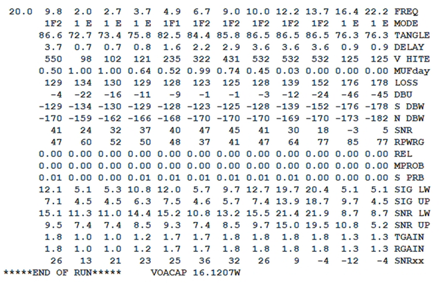
VOACAP Output
Adjusting the transmitter's frequency
The antennas on both the transmitter and receiver are designed for a frequency range of 3 - 10 MHz. This eliminates any frequencies above and below that range. You may want to focus on a frequency that has a high transmit angle (TANGLE) but a short time delay (DELAY). In this analysis, look for the best signal-to-noise ratio (SNR). This is just a sample, but for now, that will be your focus. The frequency 6.7 MHz provides a good starting point.
- Open NVIS_HF_Tx's () properties ().
- Select the Basic - Definition page when the Properties Browser opens.
- Select the Model Specs tab.
- Insert 0.0067 GHz in the Frequency field.
- Click to accept the changes and close the Properties Browser.
Refreshing the Comm Link - HF report
After changing any properties on an object that's part of a report or graph, you need to refresh the report or graph to obtain new data.
- Return to the Comm Link - HF report.
- Click Refresh (F5) (
 ) in the report's toolbar.
 - Locate the Skywave Mode column.
- Locate the Rcvd. Iso. Power (dBW) column.
- Locate the C/N (dB) column.
- When finished, close all reports, the Report & Graph Manager, and the Access Tool.
- Click Analysis in the menu bar.
- Select Remove All Accesses.
The ionosphere E layer is no longer being used.
All values are above -150.000 dBW.
There is a significant improvement. Interestingly, in the C/N (dB) column there are fluctuations in values. Your values are lowest during the hours of darkness and they are low around noon local time, where 19:00:00 (UTCG) is noon and 07:00:00 (UTCG) is midnight.
Using low-angle long-range skywaves
When high-frequency signals enter the ionosphere at a low angle, they are bent back toward the earth by the ionized layer. If the peak ionization is strong enough for the chosen frequency, a wave will exit the bottom of the layer earthward. The Earth's surface then reflects the descending wave back up again toward the ionosphere. When operating at frequencies just below the maximum usable frequency (MUF), losses can be quite small. The radio signal could skip between the earth and ionosphere two or more times (multihop propagation). Signal power of only a few Watts can sometimes be received thousands of kilometers away.
Inserting the long-range transmitter
The long-range communications link is between Los Angeles and Landstuhl, Germany.
- Insert a Transmitter () object using the Insert Default () method.
- Select Los_Angeles () in the Select Object dialog box.
- Click .
- Rename Transmitter2 () to LR_HF_Tx.
Using a Complex Transmitter model
- Open LR_HF_Tx's () properties ().
- Select the Basic - Definition page when the Properties Browser opens.
- Click the Transmitter Model Component Selector ().
- Select Complex Transmitter Model () in the Transmitter Models list in the Select Component dialog box.
- Click to close the Select Component dialog box.
Updating the model specifications
You will transmit on a frequency of 20 MHz using 100 Watts of power and a data rate of 1 Mb per second.
- Select the Model Specs tab.
- Set the following model specifications:
- Click to accept the changes and keep the Properties Browser open.
| Option | Value |
|---|---|
| Frequency | 0.02 GHz |
| Power | 100 W |
| Data Rate | 1 Mb/sec |
Specifying the long-range transmitter antenna
You want to use a custom antenna pattern for your analysis. STK Communications enables you to specify an external antenna pattern file that contains user-defined data. You will use a PhiTheta external antenna pattern file formatted to the specifications of your antenna.
- Select the Antenna tab.
- Select the Model Specs subtab.
- Click the Antenna Model Component Selector ().
- Select External Antenna Pattern () in the Antenna Models list in the Select Component dialog box.
- Click to close the Select Component dialog box.
- Click the External Filename ellipsis ().
- Go to the location of the external antenna pattern file, typically <STK install folder>\Data\Resources\stktraining\samples, in the Select File dialog box.
- Select VOACAP.pattern.
- Click .
- Insert 0.015 GHz in the Design Frequency field.
- Click to accept the changes and keep the Properties Browser open.
Changing the antenna's orientation
The antenna is directional, so point it toward your target location.
- Select the Orientation subtab.
- Enter 65 deg in the Azimuth field.
- Click to accept the changes and keep the Properties Browser open.
This will point the antenna pattern boresite in the general direction of Landstuhl, Germany.
Removing the line-of-sight (LOS) constraint
- Select the Constraints - Active page.
- Clear the Enable check box for Line Of Sight in the Active Constraints section.
- Click to accept the changes and close the Properties Browser.
Inserting a Place object to act as the long-range receiver site
Insert a Place (![]() ) object using the city database.
) object using the city database.
- Insert a Place () place object using the From City Database () method.
Selecting the long-range receiver site
The receiver site is located approximately 9480 kilometers from Los Angeles.
- Enter Landstuhl in the Name field in the Search Standard Object Data dialog box.
- Click .
- Select Landstuhl - Rheinland Pfalz - GERMANY in the Results list.
- Click .
- Click .
Inserting the long-range receiver
Attach a Receiver (![]() ) object to Landstuhl (
) object to Landstuhl (![]() ).
).
- Insert a Receiver () object using the Insert Default () method.
- Select Landstuhl () in the Select Object dialog box.
- Click .
- Rename Receiver2 () to LR_HF_Rx.
Using the Complex Receiver model
- Open LR_HF_Rx's () properties ().
- Select the Basic - Definition page when the Properties Browser opens.
- Click the Receiver Model Component Selector ().
- Select Complex Receiver Model () in the Receiver Models list in the Select Component dialog box.
- Click to close the Select Component dialog box.
Selecting the receiver's antenna
The long-range receiver uses a dipole antenna. Its design frequency covers a range of frequencies from 10 MHz through 30 MHz.
- Select the Antenna tab.
- Select the Model Specs subtab.
- Click the Antenna Model Component Selector ().
- Select Dipole () in the Antenna Models list in the Select Component dialog box.
- Click to close the Select Component dialog box.
Updating the Dipole antenna's parameters
- Set the following model specifications:
- Click to accept the changes and keep the Properties Browser open.
| Option | Value |
|---|---|
| Design Frequency | 0.02 GHz |
| Length | 9 m |
| Efficiency | 80 % |
Changing the antenna's orientation
Change the antenna orientation to horizontal.
- Select the Orientation subtab.
- Enter 0 deg in the Elevation field.
- Click to accept the changes and keep the Properties Browser open.
Removing the line-of-sight (LOS) constraint
- Select the Constraints - Active page.
- Clear the Enable check box for Line Of Sight in the Active Constraints section.
- Click to accept the changes and close the Properties Browser.
Creating an access
To determine the performance of the communication link between Los_Angeles (![]() ) and Landstuhl (
) and Landstuhl (![]() ), create an access between the LR_HF_Tx (
), create an access between the LR_HF_Tx (![]() ) and LR_HF_Rx (
) and LR_HF_Rx (![]() ).
).
- Right-click LR_HF_Tx () in the Object Browser.
- Select Access... () in the shortcut menu.
- Expand () Landstuhl () in the Associated Objects list in the Access Tool.
- Select LR_HF_Rx ().
- Click .
- Click .
Generating an HF link budget report
Determine the link performance.
- Select the Specify Time Properties option in the Time Properties panel of the Report & Graph Manager.
- Select the Use step size / time bound option.
- Enter 1 hr in the Step size field.
- Select the Comm Link - HF () report in the Installed Styles () list in the Styles panel.
- Click .
Interpreting the data providers
- Locate the Skywave Transmit Elevation column.
- Locate the Skywave Mode column.
- Locate the Rcvd. Iso. Power (dBW) column.
- Locate the C/N (dB) column.
- Leave the Comm Link - HF report open.
- Return to the Report & Graph Manager.
The transmit elevations are much lower than the NVIS elevations.
The link experiences multihop propagation in the ionosphere F layer.
You want values higher than -150.000 dBW. Your values are very poor.
You have poor carrier-to-noise ratios.
Generating a Comm Link - VOACAP files report
Use the Comm Link - VOACAP report data to improve the link.
- Select the Comm Link - VOACAP Files () report.
- Click .
- Enter 16 Apr 2024 04:00:00.000 UTCG in the Time field in the VOACAP Files dialog box.
- Click .
- When the Comm LInk - VOACAP report generates, scroll down the report to the Output File.
Unlike the NVIS analysis, the distance between Los_Angeles (![]() ) and Landstuhl (
) and Landstuhl (![]() ) creates different nighttime and daytime conditions. The analysis start time for your scenario is 12:00 pm local time in Los Angeles. In Landstuhl, the local time is nine (9) hours later or 9:00 pm. Lower frequencies work better at night. Realistically, you would choose different times throughout the analysis period to determine when to transmit your data or initiate voice communications and choose the best frequency for that transmission.
) creates different nighttime and daytime conditions. The analysis start time for your scenario is 12:00 pm local time in Los Angeles. In Landstuhl, the local time is nine (9) hours later or 9:00 pm. Lower frequencies work better at night. Realistically, you would choose different times throughout the analysis period to determine when to transmit your data or initiate voice communications and choose the best frequency for that transmission.
Add nine hours to the VOACAP Files dialog box to determine the best transmission frequency when it's 9:00 pm local time in Germany.
Adjusting the long-range transmitter frequency
The antennas on both the transmitter and receiver are designed for a frequency range of 10 - 30 MHz. This eliminates any frequencies below that range. You may want to focus on a frequency that has a low transmit angle (TANGLE) and a short time delay (DELAY). For this analysis, look for the best signal-to-noise ratio (SNR). This is just a sample, but for now, that will be your focus.
The frequency 12.2 MHz provides the best SNR within your frequency range. Since 9.0 MHz shows the best SNR, you'll set your transmitter frequency to its lowest value of 10 MHz. Obviously, you could adjust this if needed.
- Open LR_HF_Tx's () properties ().
- Select the Basic - Definition page when the Properties Browser opens.
- Enter .01 GHz in the Frequency field.
- Click to accept your change and to close the Properties Browser.
Refreshing the Comm Link - HF report
Refresh the Comm Link - HF report to obtain new data.
- Return to the Comm Link - HF report.
- Click Refresh (F5) () in the report's toolbar.
- Locate the Skywave Transmit Elevation (deg) column.
- Locate the Rcvd. Iso. Power (dBW) column.
- Locate the C/N (dB) column.
- When finished, close all reports, the Report & Graph Manager, and the Access Tool.
- Click Analysis in the menu bar.
- Select Remove All Accesses.
For the most part, daylight transmission elevation angles have increased.
More values are now above -150.000 dBW, which can help you schedule your transmission times.
There is improvement. This is just an example and there are other losses and gains affecting the link such as skywave transmit gain and skywave range. The combination of skywave loss and skywave free-space loss greatly affect the link.
Inserting a Coverage Definition object
You have analyzed an NVIS communication link and a long-range communication link. Now you will analyze communications in a large geographical area. The Coverage Definition object defines a coverage areas for analysis.
- Insert a Coverage Definition (
 ) object using the Insert Default () method.
 - Rename CoverageDefinition1 (
 ) to HF_VOACAP_Cov.
Defining the grid area of interest
Start by defining the coverage grid. Coverage analyses are based on the accessibility of assets (objects that provide coverage) and geographical areas.
- Open HF_VOACAP_Cov's () properties ().
- Select the Basic - Grid page when the Properties Browser opens.
- Open the Type drop-down menu in the Grid Area of Interest panel.
- Select LatLon Region.
- Set the following parameters:
| Option | Value |
|---|---|
| Min. Latitude | -35 deg |
| Min. Longitude | -20 deg |
| Max. Latitude | 65 deg |
| Max. Longitude | 90 deg |
Defining the grid definition
- Enter 4 deg in the Lat/Lon field in the Point Granularity panel.
- Open the drop-down menu in the Point Altitude panel.
- Select Altitude above Terrain.
- Click to accept the changes and keep the Properties Browser open.
View the coverage grid in the 2D Graphics window
- Bring the 2D Graphics window to the front.
- Center the map over the coverage grid.

Coverage Grid
Applying a grid constraint
LR_HF_Rx (![]() ) contains the constraint you want to apply to the coverage grid.
) contains the constraint you want to apply to the coverage grid.
- Return to HF_VOACAP_Cov's () properties ().
- Click in the Grid Definition panel.
- Open the Reference Constraint Class drop-down menu in the Grid Point Access Options panel when the Grid Constraints Options dialog box opens.
- Select Receiver.
- Select Landstuhl/LR_HF_Rx in the Use Object Instance list.
- Click to close the Grid Constraints Options dialog box.
- Click to accept the changes and keep the Properties Browser open.
Selecting coverage assets
Assets properties enable you to specify the STK objects used to provide coverage.
- Select the Basic - Assets page.
- Expand () Los_Angeles () in the Assets list.
- Select LR_HF_Tx ().
- Click .
- Click to accept the changes and keep the Properties Browser open.
Turning off automatically recompute accesses
STK automatically recomputes accesses every time an object on which the coverage definition depends (such as an asset) is updated. If you want control when STK computes coverage, you need to turn this off.
- Select the Basic - Advanced page.
- Clear the Automatically Recompute Accesses check box.
- Click to accept the changes and keep the Properties Browser open.
Removing the visual grid
You don't need to see the grid on the 2D and 3D Graphics windows.
- Select the 2D Graphics - Attributes page.
- Clear the Show Points check box in the Grid panel.
- Click to accept the changes and close the Properties Browser.
Using the Compute accesses tool
The ultimate goal of coverage is to analyze accesses to an area using assigned assets and applying necessary limitations upon those accesses.
- Select HF_VOACAP_Cov () in the Object Browser.
- Click CoverageDefinition in the menu bar.
- Select Compute Accesses.
Inserting a Figure of Merit object
STK enables you to specify the method by which the quality of coverage is measured using a Figure Of Merit (![]() ) object.
) object.
- Insert a Figure Of Merit (
 ) object using the Insert Default () method.
 - Select HF_VOACAP_Cov () in the Select Object dialog box.
- Click .
- Rename FigureOfMerit1 (
 ) to Rcvd_Iso_Pwr.
Measuring access constraints
Access Constraints measure the value of various constraint parameters used to define visibility within STK.
- Open Rcvd_Iso_Pwr's () properties ().
- Select the Basic - Definition page when the Properties Browser opens.
- Set the following in the Definition panel:
- Click to accept the changes and keep the Properties Browser open.
| Option | Value |
|---|---|
| Type | Access Constraint |
| Constraints | RcvdIsotropicPower |
| Compute | Maximum |
| Time Step | 3600 sec |
Using the Overall Value by Time data provider
The Overall Value by Time Data Provider reports statistical information on time-dependent values. Statistics are generated by sampling values from all grid points at the reported times.
- Right-click Rcvd_Iso_Pwr () in the Object Browser.
- Select Report & Graph Manager... (
 ) in the shortcut menu.
 - Select the Grid Stats Over Time (
 ) graph in the Installed Styles () folder.
 - Click . Be patient, this can take a few minutes.
- Place your cursor over the lowest minimum point in the graph and read the results: approximately -448 (dBW).
- Place your cursor over the highest maximum point in the graph and read the results: approximately -124 (dBW).
- Close the Grid Stats Over Time graph and the Report & Graph Manager.
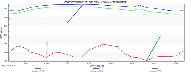
Grid Stats Over Time Graph
You can use the graph to quickly find the lowest and highest received isotropic power (dBW) values during the 24-hour analysis.
You will use these values to create contours on your 2D and 3D Graphics windows.
Defining animation graphics for the Figure Of Merit
The Animation page enables you to define animation graphics for the Figure Of Merit.
- Return to Rcvd_Iso_Pwr's () properties ().
- Select the 2D Graphics - Animation page.
- Enter 50 in the % Translucency field in the Show Points As panel.
Setting contour values
- Select the Show Contours option in the Display Metric panel.
- Set the following values:
- Click .
- Ensure Color Method is set to Color Ramp in the Level Attributes panel.
- Set Start Color to red.
- Set End Color to blue.
- Click to accept the changes and keep the Properties Browser open.
| Option | Value |
|---|---|
| Start | -450 dBW |
| Stop | -130 dBW |
| Step | 40 dBW |
You rounded down the lowest and highest values obtained from the Grid Stats Over Time (![]() ) graph.
) graph.
Creating an embedded legend
You can place legends in the 2D and 3D Graphics windows. These come in handy if using STK for a briefing or creating images for documentation.
- Click .
- Click in the Animation Legend for Rcvd_Iso_Pwr floating legend.
- Set the following values in the Figure of Merit Legend Layout dialog box:
- Click to close the Figure of Merit Legend Layout dialog box.
- Close the Animation Legend for Rcvd_Iso_Pwr floating legend.
- Click to accept the changes and close the Properties Browser.
| Option | Value |
|---|---|
| 2D Graphics Window - Show at Pixel Location | enabled |
| 3D Graphics Window - Show at Pixel Location | enabled |
| Text Options - Title | Received Isotropic Power (dBW) |
| Text Options - Number Of Decimal Digits | 0 |
| Range Color Options - Color Square Width (pixels) | 60 |
Viewing 2D Graphics window contours
Although you can view the received isotropic power (dBW) contours in both the 2D and 3D Graphics windows, due to the large geographic coverage area, it is easier to see in the 2D Graphics window.
- Bring the 2D Graphics window to the front.
- Click Increase Time Step (
 ) in the Animation toolbar to set Time Step to 3600 sec.
 - Click Start (
 ) to animate the scenario. Be patient. Each step forward will take a moment to render the next view.
 - Click Reset (
 ) when finished.
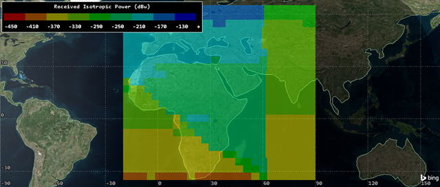
2D Graphics Window Animation Contours
Saving your work
- Close all open reports, properties, and tools.
- Save () your work.
Summary
During this tutorial, you performed three HF analyses:
- The first analysis took place between two sites, approximately 60 kilometers apart, using a high-angle skip. You employed horizontal dipole antennas at both sites. After analyzing the first link, using VOACAP files, you determined a lower frequency was required, which significantly improved communications.
- The second analysis featured a long-distance, low-angle, multihop propagation using an external directional antenna pattern on the transmitter and a dipole receiver antenna. Again, using VOACAP files, you lowered the frequency and improved the communications link.
- For the third analysis, you employed a long-distant transmitter and receiver to perform wide-area coverage, focusing on received isotropic power.
On your own
Throughout the tutorial, hyperlinks were available that pointed to in-depth information concerning Transmitter (![]() ) and Receiver (
) and Receiver (![]() ) objects. Now is a good time to go back through this tutorial and view that information. Open the VOACAP.pattern file with Notepad to understand the setup of the external antenna pattern. Go to the different receivers and transmitters properties and open the 3D Graphics - Attributes pages. Turn on and view Volume Graphics - Show Volume to view the antenna pattern in the 3D Graphics window. Try using vertical vice horizontal dipole antennas. Adjust the azimuth of the long-range transmitter's antenna and see how that affects coverage.
) objects. Now is a good time to go back through this tutorial and view that information. Open the VOACAP.pattern file with Notepad to understand the setup of the external antenna pattern. Go to the different receivers and transmitters properties and open the 3D Graphics - Attributes pages. Turn on and view Volume Graphics - Show Volume to view the antenna pattern in the 3D Graphics window. Try using vertical vice horizontal dipole antennas. Adjust the azimuth of the long-range transmitter's antenna and see how that affects coverage.