STK Premium (Space) or STK Enterprise
You can obtain the necessary licenses for this tutorial by contacting AGI Support at support@agi.com or 1-800-924-7244.
Required product install:installation of the Spectrum Analyzer Plugin, which is included with
The results of the tutorial may vary depending on the user settings and data enabled (online operations, terrain server, dynamic Earth data, etc.). It is acceptable to have different results.
Capabilities covered
This lesson covers the following capabilities of the Ansys Systems Tool Kit® (STK®) digital mission engineering software:
- STK Pro
- Communications
- STK SatPro
Problem statement
Engineers and operators must be mindful of potential sources of interference to their communications links. A new satellite internet constellation of low Earth orbit (LEO) satellites is being proposed that will transmit data within the 12-18 gigahertz Ku band. Many maritime very-small-aperature terminal (VSAT) communication systems also operate in this portion of the electromagnetic spectrum. You want to determine if any of the LEO satellites will interrupt the transfer of data between a satellite in geosynchronous orbit (GEO) and the VSAT system on a ship at sea.
Solution
Use the STK software's Communications capability to compute a link budget between the shipboard receiver using a phased array antenna and a GEO satellite. Then, use the SatPro capability's Walker tool to model a portion of the proposed constellation of LEO satellites. Use the Spectrum Analyzer plugin to view the spectrum utilization and visualize potential interference on the communication link to determine if any of the LEO satellites interrupt data transfer between the GEO satellite and the ship. Finally, add nulls to the phased array antenna to view the effects.
What you will learn
Upon completion of this tutorial, you will be able to:
- Analyze communication interference
- Use the Spectrum Analyzer to determine interference sources
Creating a new scenario
First, create a new scenario, the build from there.
- Launch the STK application (
 ).
). - Click
 Create a Scenario when the Welcome to STK dialog box opens.
 - Enter the following in the New Scenario Wizard:
- Click when you are done.
- Click Save (
 ) once the scenario loads.
 - Verify the scenario name and location and click .
| Option | Value |
|---|---|
| Name | SpectrumAnalyzer |
| Start | Date: Default / Time: 19:00:00.000 UTCG |
| Stop | + 2 hrs |
A folder with the same name as your scenario is created for you.
Save (![]() ) often during this tutorial!
) often during this tutorial!
Disabling streaming terrain
Streaming terrain is not required for this analysis. Disable the Terrain Server.
- Right-click on SpectrumAnalyzer () in the Object Browser.
- Select Properties (
 ) in the shortcut menu.
 - Select the Basic - Terrain page when the Properties Browser opens.
- Clear the Use terrain server for analysis check box in the Terrain Server panel.
- Click to confirm your change and to close the Properties Browser.
Inserting the GEO satellite
Insert a Satellite object, which will function as the GEO communications satellite.
- Bring the Insert STK Objects tool (
 ) to the front.
 - Select Satellite (
 ) in the Select An Object To Be Inserted list.
 - Select Orbit Wizard (
 ) in the Select A Method list.
 - Click .
- Set the following options when the Orbit Wizard opens:
- Leave all other settings at their default values.
- Click to propagate GEO_Sat () and to close the Orbit Wizard.
| Option | Value |
|---|---|
| Type | Geosynchronous |
| Satellite Name | GEO_Sat |
Modeling the GEO satellite's transmitter
Model the transmitter on board the satellite and configure its properties.
Inserting a Transmitter object
Insert a
- Bring the Insert STK Objects tool () to the front.
- Insert a Transmitter (
 ) object using the Insert Default () method.
 - Select GEO_Sat () when the Select Object dialog box opens.
- Click to confirm your selection and to close the Select Object dialog box.
- Right-click on Transmitter1 () in the Object Browser.
- Select Rename in the shortcut menu.
- Rename Transmitter1 () GEO_Tx.
Using a Complex Transmitter model
Use a Complex Transmitter model for the transmitter. A
- Open GEO_Tx's () Properties ().
- Select the Basic - Definition page when the Properties Browser opens.
- Click the Transmitter Model Component Selector (
 ).
). - Select Complex Transmitter Model (
 ) when the Select Component dialog box opens.
 - Click to confirm your selection and to close the Select Component dialog box.
- Click to confirm your change and to keep the Properties Browser open.
Modeling a parabolic antenna
The satellite is equipped with a parabolic antenna. Use the
- Select the Antenna tab.
- Select the Model Specs sub-tab.
- Click the Antenna Model Component Selector ().
- Select Parabolic () when the Select Component dialog box opens.
- Click to confirm your selection and to close the Select Component dialog box.
- Enter 2 m in the Diameter field.
- Click to confirm your changes and to keep the Properties Browser open.
The installed
Updating the antenna orientation
The STK application provides
- Select the Orientation sub-tab.
- Set the following parameters:
- Click to confirm your changes and to keep the Properties Browser open.
| Option | Value |
|---|---|
| Azimuth | 244.0529 deg |
| Elevation | 83.92558 deg |
Setting the transmitter's modulation options
The Communications capability allows you to set the transmitter's modulation options. The Power Spectral Density (PSD) option allows the Communications capability to model the actual spectral shape of the transmitted signal based on the modulation, data rate, etc.
- Select the Modulator tab.
- Select the Use Signal PSD check box.
- Set the Number of Spectrum Nulls to 3.
- Click to confirm your changes and to close the Properties Browser.
The number of nulls will automatically set the signal's bandwidth.
Modeling the ship
The ship is anchored off the coast of California. It will function as the test location for satellite communications reception.
Inserting a new Ship object
Insert a
- Bring the Insert STK Objects tool () to the front.
- Insert a Ship object (
 ) using the Insert Default () method.
 - Rename Ship1 () Ship.
Defining the ship's route options
The ship is located off the coast of California.
- Open Ship's () Properties ().
- Select the Basic - Route page when the Properties Browser opens.
- Use the default GreatArc propagator.
- Open the Route Calculation Method drop-down list.
- Select Specify Time.
- Open the Reference drop-down list in the Altitude Reference panel.
- Select WGS84.
The ship will remain stationary for two hours. Specify Time uses the Time properties of each waypoint.
Since you've disabled analytical terrain, you want the ship to sit on the surface of the WGS84 ellipsoid.
Defining the ship's waypoints
Now, add the waypoints for the ship's route. The ship will remain stationary, so you can define a route using two waypoints set at the same location over the course of your analysis period.
- Click .
- Set the following options for the first waypoint:
- Click again.
- Set the second waypoint's time to be two hours from the first point's time (for example, [Date] 21:00:00.000 UTCG).
- Click to confirm your changes and to close the Properties Browser.
| Option | Value |
|---|---|
| Latitude | 33.65 deg |
| Longitude | -119.56 deg |
You want to be sure the ship remains stationary for the duration of your analysis period.
Updating the 2D Graphics window properties
Configure the 2D Graphics window to improve situational awareness.
Removing the background image
You can remove the background image (a Microsoft Bing map or image file) by updating the
- Bring the 2D Graphics window to the front.
- Click Properties () on the 2D Window Defaults toolbar.
- Select the Imagery page when the Properties Browser opens.
- Clear the Show check box in the Background Image panel.
- Click to confirm your change and to keep the Properties Browser open.
Selecting map details
Update the map details to display additional borders in the 2D Graphics window.
- Select the Details page.
- Click to select the following options in the Map Details list:
- RWDB2_Coastlines (selected by default)
- RWDB2_International_Borders
- RWDB2_Islands
- RWDB2_Provincial_Borders
- Click to confirm your selections and to close the Properties Browser.
Viewing the ship in relation to the satellite antenna's boresight
The GEO satellite antenna is boresighted on (that is, the antenna is orientated towards) the California coast. The ship is approximately 67 kilometers away from this location at a bearing of 219 degrees. You can see the ship and the antenna's
- Bring the 2D Graphics window to the front.
- Zoom in to the map so that you can see the Ship object and a small (X) on the California coast, which pinpoints the antenna boresight.
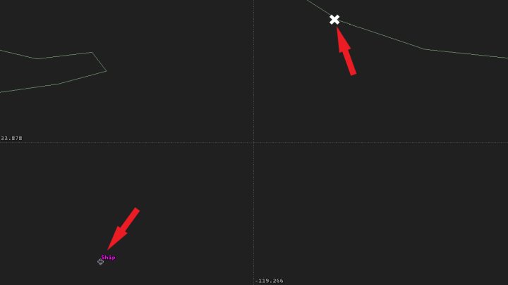
Antenna Boresight (The Boresight marker has been bolded for clarity)
Modeling the ship's receiver
Model the ship's onboard VSAT receiver and configure its properties.
Inserting a Receiver object
Insert a
- Bring the Insert STK Objects tool () to the front.
- Insert a Receiver (
 ) object using the Insert Default () method.
 - Select Ship () when the Select Object dialog box opens.
- Click to confirm your selection and to close the Select Object dialog box.
- Rename Receiver1 () Ship_Rx.
Using a Complex Receiver model
A
- Open Ship_Rx's () Properties ().
- Select the Basic - Definition page when the Properties Browser opens.
- Click the Receiver Model Component Selector ().
- Select Complex Receiver Model () when the Select Component dialog box opens.
- Click to confirm your selection and to close the Select Component dialog box.
- Clear the
- Keep the default frequency of 14.5 GHz.
- Click to confirm your changes and to keep the Properties Browser open.
Using a Phased Array antenna model
The ship is equipped with a phased array antenna containing 19 elements. A
- Select the Antenna tab.
- Select the Model Specs sub-tab.
- Click the Antenna Model Component Selector ().
- Select Phased Array () when the Select Component dialog box opens.
- Click to confirm your selection and to close the Select Component dialog box.
Setting the element configuration
The Element Configuration tab enables you to define the physical aspects of the antenna elements. Use the default Hexagon element configuration, which represents a two-dimensional planar antenna array with an aperture shape consisting of six sides and a triangular stricture, which staggers the elements between rows and columns.
- Select the Element Configuration sub-tab on the Model Specs sub-tab.
- Set the following values in the Number of Elements panel:
- Click to confirm your changes and to keep the Properties Browser open.
| Option | Value |
|---|---|
| X | 5 |
| Y | 5 |
Target the geosynchronous satellite
The Beam Direction Provider tab enables you to select where the antenna points its beam. The phased array antenna elements will track the GEO satellite.
- Select the Beam Direction Provider sub-tab on the Model Specs sub-tab.
- Select the Enabled check box in the Beam Steering panel.
- Select GEO_Sat () in the Available Objects list.
- Move (
 ) GEO_Sat () to the Assigned Objects list.
 - Click to confirm your changes and to keep the Properties Browser open.
Defining the receiver's bandwidth
Enter a value for the receiver's bandwidth by clearing the Auto Scale option.
- Select the Filter tab at the top of the page.
- Clear the Auto Scale check box in the Receiver Bandwidth panel.
- Enter 96 MHz in the Bandwidth field.
- Click to confirm your change and to keep the Properties Browser open.
Displaying the antenna volume graphics
Volume graphics allow you to display the shape and gain levels of antenna beams. The receiver's
- Select the 3D Graphics - Attributes page.
- Select the Show Volume check box in the Volume Graphics panel.
- Enter -10 dB in the Minimum Displayed Gain field.
- Select the Set azimuth and elevation resolution together check box in the Pattern panel.
- Enter 1 deg in the Resolution field in the Azimuth panel.
- Click to confirm your changes and to close the Properties Browser.
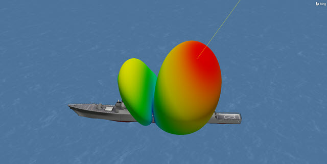
Viewing Ship_Rx's antenna pattern in the 3D Graphics window
You can view the phased array antenna pattern in the 3D Graphics window and the access to GEO_Sat.
- Bring the 3D Graphics window to the front.
- Zoom to Ship ().
- Use your mouse to obtain a view of the phased array antenna pattern.
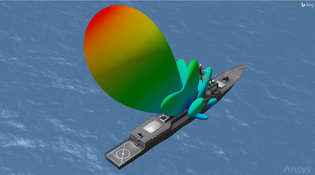
phased array antenna pattern
Evaluating the communications link
The STK Communications capability allows you to model and
Computing access
You can model a communications link by computing access between a transmitter and a receiver with the
- Right-click on Ship_Rx () in the Object Browser.
- Select Access... (
 ) in the shortcut menu.
 - Expand (
 ) GEO_Sat () in the associated objects list when the Access tool opens.
 - Select GEO_Tx ().
- Click
 .
.
Generating a link budget report
A Link Budget report includes all the link parameters associated with the selected receiver or transmitter. Generate a Link Budget report between the ship and the GEO satellite using the Link Budget button in the Reports panel of the Access tool.
- Click in the Reports panel.
- Scroll to the right of the report and note the Eb/No (dB) values.
- Close the Link Budget report and the Access tool when you are finished.
The Eb/No, the signal-to-noise ratio at the receiver, is what you'll focus on throughout the tutorial.
Creating the LEO satellite constellation with the Walker tool
Model the constellation of LEO satellites by using the Walker tool. The Walker tool, available with the SatPro capability, makes it easy to generate a Walker constellation using the Two Body, J2, J4, or SGP4 orbit propagators The original satellite that is used to create the Walker constellation is referred to as the "seed" satellite, while the satellites generated using the Walker tool are referred to as children.
A Walker constellations is based on a simple design strategy for distributing the satellites in a constellation. Its consists of a group of satellites (t) that are in circular orbits and have the same period and inclination. The pattern of the constellation consists of evenly spaced satellites (s) in each of the orbital planes (p) specified so that t = sp. The ascending nodes of the orbital planes are also evenly spaced over a range of right ascensions (RAAN).
Inserting the seed satellite
Use the Orbit Wizard to create the "seed" satellite from which the other satellites will be derived. When you create a Walker constellation, the tool duplicates the original (seed) satellite as part of the constellation. The new satellites will be children of this seed.
- Bring the Insert STK Objects tool () to the front.
- Insert a Satellite () object using the Orbit Wizard () method.
- Set the following options when the Orbit Wizard opens:
- Click to propagate LEO_Sat () and to close the Orbit Wizard.
| Option | Value |
|---|---|
| Type | Sun Synchronous |
| Satellite Name | LEO_Sat |
Leave all other settings at their default values.
Attaching a Sensor object for situational awareness
When a seed satellite has attached child objects such as sensors and transmitters, the Walker tool creates the same sub-objects for each of the child satellites; that is, the Walker Tool will copy them into the constellation. Attach a Sensor object to your LEO seed satellite. Its field of view, which will encompass the antenna beams, is for operator situational awareness.
- Bring the Insert STK Objects tool () to the front.
- Insert a Sensor (
 ) object using the Define Properties () method.
 - Select LEO_Sat () when the Select Object dialog box opens.
- Click to confirm your selection and to close the Select Object dialog box.
- Select the Basic - Definition page when the Properties Browser opens.
- Set the following options:
- Click to confirm your changes and to keep the Properties Browser open.
| Option | Value |
|---|---|
| Sensor Type | Simple Conic |
| Cone Half Angle | 2.8 deg |
Orienting the Sensor object
The Fixed pointing type enables you to specify the orientation of the sensor with respect to the body frame of your parent object. While the sensor remains fixed relative to the parent object, motion of the parent object changes the direction in which the sensor is pointing.
- Select the Basic - Pointing page.
- Set the following options in the Fixed panel:
- Click to confirm your changes and close the Properties Browser.
- Rename Sensor1 () Sensor.
The default Pointing type is Fixed.
| Option | Value |
|---|---|
| Azimuth | 90 deg |
| Elevation | 85 deg |
Inserting a Transmitter object
Attach a transmitter object to Sensor.
- Bring the Insert STK Objects tool () to the front.
- Insert a Transmitter () object using the Insert Default () method.
- Select Sensor () when the Select Object dialog box opens.
- Click to confirm your selection and to close the Select Object dialog box.
- Rename Transmitter2 () LEO_Xmtr.
Defining the LEO satellite transmitter's properties
Each LEO satellite has 18 transmitter beams. The Multibeam Transmitter model enables you to set up multiple antenna beams, each with its own specs and its own polarization and orientation properties.
- Open LEO_Xmtr's (
 ) Properties ().
 - Select the Basic - Definition page when the Properties Browser opens.
- Click the Transmitter Model Component Selector ().
- Select Multibeam Transmitter Model () when the Select Component dialog box opens.
- Click to confirm your selection and to close the Select Component dialog box.
Setting the modulation options
Use the Power Spectral Density (PSD) option.
- Select the Modulator tab.
- Select the Use Signal PSD check box.
- Set the Number of Spectrum Nulls to 3.
- Click to confirm your changes and to keep the Properties Browser open.
Setting the beam and antenna properties
Use the Beams tab to define parameters for the antenna's beams. The Beams tab contains a Beam summary table, a Beam Selection Strategy field, and two additional rows of tabs: one for beam parameters, and one for antenna parameters.
- Select the Beams tab.
- Select the Beam Specs sub-tab.
- Enter 14.51 GHz in the Frequency field.
- Select the Antenna sub-tab.
- Select the Model Specs sub-tab in the Antenna sub-tab.
- Enter 14.51 GHz in the Design Frequency field.
- Select the Orientation sub-sub in the Antenna sub-tab.
- Set the following orientation parameters:
- Click to confirm your changes and to keep the Properties Browser open.
| Option | Value |
|---|---|
| Azimuth | 0 deg |
| Elevation | 89 deg |
Defining the antenna beams
Use the beam summary table to perform an Add, Duplicate, Remove, and Orient operations on one or more beams.
- Select Beam001 in the Beam Summary Table.
- Click seventeen times so that you have a total of eighteen beams in the list.
A Beam ID is automatically assigned to each copied beam. You should see Beam001 through Beam018 in the table.
Adjusting the beams' orientation
Adjust the beams' orientation by batch editing them in two groups.
- Select Beam001.
- Hold down the Shift key.
- Select Beam006 to multi-select all six beams.
- Click .
- Set the following values when the Antenna Beam Orientation dialog box opens:
- Click to confirm your changes and to close the Antenna Beam Orientation dialog box.
| Orientation | Initial Value | Increment Value |
|---|---|---|
| Elevation | 89 deg | 0 deg |
| Azimuth | 0 deg | 60 deg |
Adjusting the second group of beams' orientation
Now, orient the second group.
- Select Beam007.
- Hold down the Shift key.
- Select Beam018 to multi-select all 12 beams.
- Click .
- Set the following values when the Antenna Beam Orientation dialog box opens:
- Click to confirm your changes and to close the Antenna Beam Orientation dialog box.
- Confirm your beams are oriented as shown in the below table:
- Click to confirm your changes and close the Properties Browser.
| Orientation | Initial Value | Increment Value |
|---|---|---|
| Elevation | 88 deg | 0 deg |
| Azimuth | 0 deg | 30 deg |
| Beam ID | Azimuth | Elevation |
|---|---|---|
| Beam001 | 0 deg | 89 deg |
| Beam002 | 60 deg | 89 deg |
| Beam003 | 120 deg | 89 deg |
| Beam004 | 180 deg | 89 deg |
| Beam005 | 240 deg | 89 deg |
| Beam006 | 300 deg | 89 deg |
| Beam007 | 0 deg | 88 deg |
| Beam008 | 30 deg | 88 deg |
| Beam009 | 60 deg | 88 deg |
| Beam010 | 90 deg | 88 deg |
| Beam011 | 120 deg | 88 deg |
| Beam012 | 150 deg | 88 deg |
| Beam013 | 180 deg | 88 deg |
| Beam014 | 210 deg | 88 deg |
| Beam015 | 240 deg | 88 deg |
| Beam016 | 270 deg | 88 deg |
| Beam017 | 300 deg | 88 deg |
| Beam018 | 330 deg | 88 deg |
You can also generate an Antenna Properties report for LEO_Xmtr to double-check if the Beam values match the table.
Creating the Walker constellation from the seed satellite
With your seed satellite and its attached objects created, use the Walker tool to create the LEO constellation. When you create a Walker constellation, the tool duplicates the seed satellite as part of the constellation. The new satellites will be children of the seed, and child will the same base name as the seed satellite plus two numbers: the first number identifies the plane in which the satellite resides, and the second identifies the satellite's position in the plane.
- Right-click on LEO_Sat () in the Object Browser.
- Select Satellite in the Shortcut menu.
- Select Walker... in the Satellite submenu.
- Set the following options when the Walker tool opens:
- Click .
- Click after the satellites have been propagated and to close the Walker tool.
- Save () your scenario.
| Option | Value |
|---|---|
| Type | Delta |
| Number of Sats Per Plane | 10 |
| Number of Planes | 2 |
| Interplane Spacing | 1 |
| Color by Plane | Cleared |
When you save the scenario, all objects in the scenario are also saved. It is important that you save the scenario before you remove the seed satellite in case you need to reload your scenario later for further analysis.
Removing the seed satellite
You do not need LEO_Sat for your analysis. You can remove it from your scenario.
- Select LEO_Sat () in the Object Browser.
- Click Delete (
 ) on the Object Browser toolbar.
 - Click when the Delete Object dialog box opens to confirm your delete and to remove LEO_Sat and its attached sensor and transmitter from your scenario.
Viewing the LEO satellite constellation
View the constellation of LEO satellites in the 3D Graphics window.
- Bring the 3D Graphics window to the front.
- Click Home View (
 ) in the 3D Graphics window's 3D Graphics toolbar.
 - Use your mouse to turn the Earth in order to view the constellation of LEO satellites.
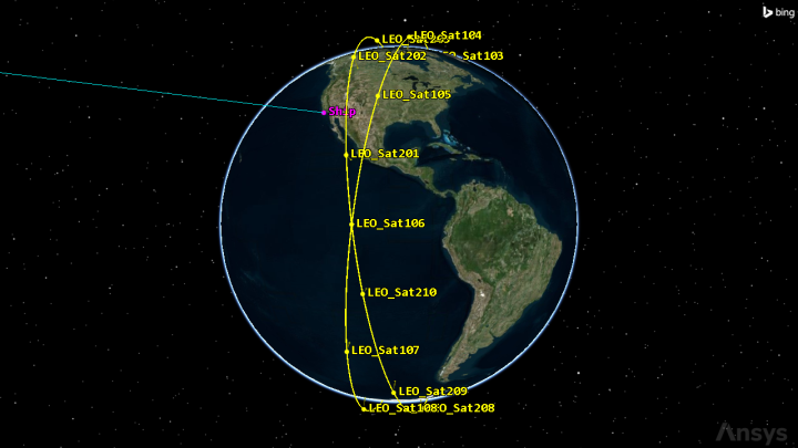
LEO Satellite Constellation
Cleaning up the 2D and 3D Graphics windows view
You can remove the satellites' ground tracks and orbits to declutter your view by updating the scenario's
- Open SpectrumAnalyzer's () Properties ().
- Select the 2D Graphics - Global Attributes page when the Properties Browser opens.
- Clear the Show Ground Tracks/ Routes and Show Orbits/ Trajectories check boxes in the Vehicles panel.
- Click to confirm your changes and to close the Properties Browser.
Adding interference sources to the receiver
You can add interference sources in Ship_Rx's properties. Then, you can assess their impact on the performance of Ship_Rx.
- Open Ship_Rx's () Properties ().
- Select the Basic - Definition page when the Properties Browser opens.
- Select the Interference tab.
- Select the Use check box.
- Select the Transmitter () check box in the Selection filter panel.
- Move () all the Transmitter objects to the Assigned Emitters list.
- Remove (
 ) GEO_Sat/GEO_Tx () from the Assigned Emitters list.
 - Click to confirm your changes and to close the Properties Browser.
Evaluating the impact of RF interference
Determine if RF interference is affecting the ship's reception and to what extent.
Creating a new custom graph style
Use the Report & Graph Manager to create a
- Click Report & Graph Manager... (
 ) in the Data Providers toolbar.
 - Open the Object Type drop-down list when the Report & Graph Manager opens.
- Select Access.
- Select Ship-Ship-Receiver-Ship_Rx-To-Satellite-GEO_Sat-Transmitter-GEO_Tx (
 ) in the Object Type list.
 - Select the My Styles (
 ) folder in the Style list panel.
 - Click Create new graph style (
 ) in the Styles toolbar.
 - Name the new graph EbNo Interference (
 ).
). - Select the Enter key.
Selecting the data provider elements
Use Link Information data provider elements for your custom graph. Link information provides the link budget for a single access between a transmitter and a receiver.
- Expand () the Link Information () data provider in the Data Providers list when the Properties Browser opens.
- Select the Eb/No (
 ) data provider element.
 - Move () Eb/No () to the Y Axis list.
- Select Eb/(No+Io) () in the Data Providers list.
- Move () Eb/(No+Io) () to the Y Axis list.
- Enter 1.000 sec in the Step Size field in the Step Size panel.
- Click to confirm your changes and to close the Properties Browser.
This is the energy per bit-to-noise ratio.
This is the energy per bit-to-noise-plus-interference ratio.
Placing both elements in the Y Axis makes the graph easier to read.
Generating the custom graph
Generate your custom graph to visualize the effects of interference on the signal between the ship and the GEO satellite.
- Select EbNo Interference () in the My Styles () folder.
- Click .
- Using the left mouse button, zoom in on the first spike in the graph.
- Right-click on the bottom of the spike.
- Select Set Animation Time in the shortcut menu.
- Keep the EbNo Interference graph open.
- Close the Report & Graph Manager.
Depending on your computer, this could take a minute or two. You can monitor the execution with the Progress Bar, located in the Status Bar at the bottom of the STK workspace.
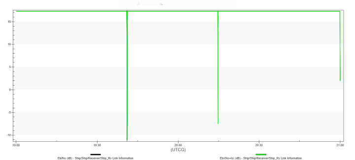
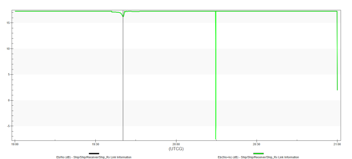
Eb/No Interference
You can see that there are several times when LEO satellite transmissions could potentially interfere with the ship's reception of the GEO satellite transmission.
If needed, go to the graph's toolbar and click Toggle animation time line (![]() ) in order to see the vertical time line in the graph.
) in order to see the vertical time line in the graph.
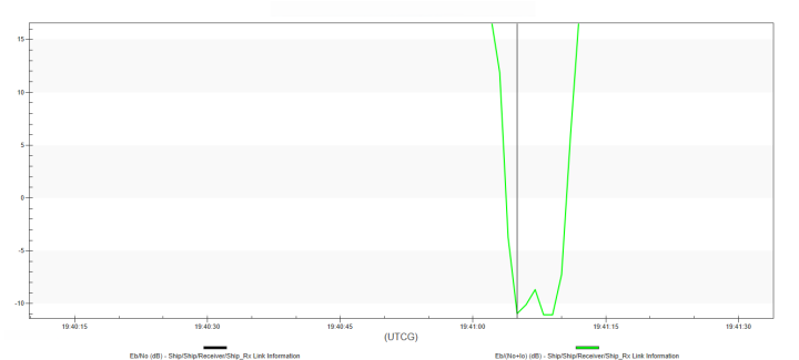
Eb/No with Time Line
Using the Spectrum Analyzer
The Spectrum Analyzer is similar in nature to a real spectrum analyzer instrument, but with some additional features tailored toward the STK application. The Spectrum Analyzer plugin enables you to view the spectrum utilization in different ways. It has various modes to help you understand the currently assigned emitter frequency allocations as well as when and how "hot" the spectrum band is currently being utilized. You can visualize the aggregate spectrum utilization and intensity from the perspective of what a specific receiver, at some geographical position, may encounter. It can show the emitters as itemized power spectrum densities at an instantaneous time or as an aggregate over a window of time.
Opening the Spectrum Analyzer
Open the Spectrum Analyzer plugin from the Spectrum Analyzer toolbar. The toolbar ( ) contains one icon. Clicking the icon will launch a new instance of the Spectrum Analyzer.
- Select View on the Menu bar.
- Select the Toolbars menu.
- Select Spectrum Analyzer in the Toolbars submenu.
- Click Spectrum Analyzer (
 ) on the Spectrum Analyzer Toolbar.
Selecting GEO_Tx for display
The Transmitters panel displays the names of all the transmitters within the scenario.
- Adjust the size of the Spectrum Analyzer window to see the full extent of the tool, if necessary, to view the Transmitters panel.
- Select the check box for /Satellite/GEO_Sat/Transmitter/GEO_Tx in the Transmitters panel when the Spectrum Analyzer opens.
Enabling Receiver View
You want to analyze the interference from the point of view of the receiver on board the ship. The Receiver panel displays the names of all the receivers within the scenario, which are neither Bandwidth Auto-scaled nor have Frequency Auto-Tracking enabled. Enabling Receiver View automatically adjusts the Sweep Display panel to show the frequency band that is seen by the selected receiver, provided that Lock To Receiver is also selected; it is as if the Spectrum Analyzer was sitting at the receiver's location.
- Select the Receiver View check box.
- Confirm the Lock To Receiver check box is selected.
The Lock To Receiver check box is provided in the event that you want to change the band to "inspect" what is happening in an area of the spectrum outside the receiver.
When Receiver View is selected, the powers displayed are before the receiver electronics, and thus will include spatial aspects, propagation effects, Doppler, antenna gain, and polarization.
If you have left have left Ship_Rx's Bandwidth Auto Scale check box and/or its Frequency Auto Track check box selected, Receiver View will be disabled.
Adjusting the Data Display
The Data Display panel displays important information and values associated with each time step. There are two items that are always displayed (the time and the contention, which will display YES when two transmitters overlap in their frequency bands) as well as a set of items that can be selected for display. The peak value of each sweep (in dB) is already enabled to be shown on the Data Display. Add the carrier-to-interference ratio (C/I) to the data display to display.
- Select Data Display in the Spectrum Analyzer menu bar.
- Select C/I in the Data Display submenu.
Updating the Sweep Display
The Sweep Display panel displays Sweeps that represent various views of a signal. The Sweep Display panel's horizontal axis represents the frequency. The vertical axis depends on the selected display mode. In this case, you want to use the default Power Spectral Density mode, which sweeps at each time step (in dBW). The displayed sweeps represent the Power Spectral Density that the receiver will see at the input to the receiver back-end electronics, which was set when you checked Receiver View. The horizontal axis displays information, which includes lower frequency limit (Fl), upper frequency limit (Fu), center frequency (Fc), and bandwidth (BW). Increase the thickness of the drawn sweeps and the vertical scale for easier viewing on the Sweep Display.
- Select the Edit menu on the Spectrum Analyzer menu bar.
- Select Properties... in the Edit submenu.
- Increase the Sweep Line Width to 3 when the Properties dialog box opens.
- Click to confirm your change and to close the Properties dialog box.
- Use the Vertical Scale knob to set the Vertical Scale to approximately -160.
If it hasn't displayed already, this will refresh the Data Display to show C/I (in dB).
You can also enter -160 in the Vertical Scale field and select the Tab key to set the value exactly.
Determining which transmitter is interfering with your receiver
You have determined that there are a few instances of possible interference and you've set your scenario to the time of the first interference. Now you can use the Spectrum Analyzer to determine which LEO transmitter is interfering with your system.
- In the Transmitters list, start selecting each check box until you see a second signal overlapping the original signal in the data display.
- Right-click on /Satellite/LEO_Sat207/Sensor/Sensor18/Transmitter/LEOXmtr17 in the Transmitters list.
- Select Red when the Color dialog box opens.
- Click to confirm your selection and to close the color dialog box.
If you focused on the first spike in the custom graph, you should see the transmission from /Satellite/LEO_Sat207/Sensor/Sensor18/Transmitter/LEOXmtr17 is interfering with your communications.
After changing the color of the transmitter, the next time the sweep is drawn it will be drawn in the new color. When the transmitter's sweep color is changed, it only changes the color within the Spectrum Analyzer, it will not change the color being used by the STK object's 2D and 3D graphics.
Animating the scenario
Animate the scenario to view the interference in action.
- Click Decrease Time Step (
 ) in the Animation toolbar and set the time step to 0.10 sec.
 - Bring your EbNo Interference graph to the front.
- Click Zoom Out (
 ) until you can see the whole graph.
 - Zoom in at the top of the period that interference is taking place.
- Right click on the graph when the interference is just beginning.
- Select Set Animation Time in the shortcut menu.
- Bring the Spectrum Analyzer back to the front.
- Click Start (
 ) in the animation toolbar to animate the scenario.
 - Watch as the interference dominates the desired signal for a short amount of time in the Sweep Display.
- Click Pause (
 ) during a time when the interference is dominating.
First Interference Period
![]()
LeoXmtr17 Dominates GEO_Tx
Visualizing the beams in 2D
You can view the satellite's antenna beams in the 2D Graphics window by updating the attached transmitter's
- Open LEO_Xmtr17's () Properties ().
- Select the 2D Graphics - Contours page when the Properties Browser opens.
- Select the Show Contour Graphics check box.
- Make the following changes in the Level Adding panel:
- Click .
- Change the Start Color to Red in the Level Attributes panel.
- Change the Stop Color to Blue.
- Select the Set azimuth and elevation resolution together check box.
- Set the Resolution to 1 deg in the Azimuth panel.
- Click to confirm your changes and to keep the Properties Browser open.
LEO_Xmtr17 is attached to LEO_Sat207.
| Option | Value |
|---|---|
| Start | -3 |
| Stop | 0 |
| Step | 3 |
Enabling 3D contour graphics
Update the transmitter's
- Select the 3D Graphics - Attributes page.
- Select the Show Lines check box in the Contour Graphics panel.
- Click to confirm your changes and close the Properties Browser.
- Save () your scenario.
Viewing the antenna beams in 3D
View the beams in the 3D Graphics window.
- Bring the 3D Graphics window to the front.
- Zoom To LEO_Sat207 ().
- Use the mouse buttons to move your view.
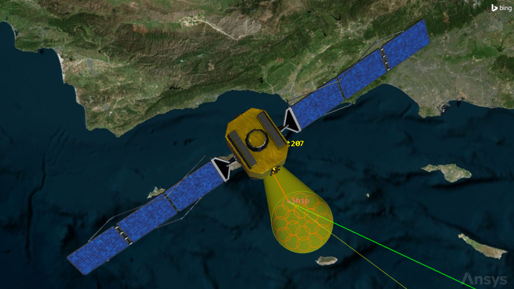
3D View Multibeam Transmitter Pattern
You can see the antenna beam crosshairs inside the simple conic sensor's field of view. As the satellite passes over Ship, the Spectrum Analyzer shows at least some of the beams are interfering with your communications.
Incorporating nulls into the phased array antenna
A phased array antenna not only can steer its maximum gain in a particular direction, but it can also steer nulls toward other directions to prevent radiation to and from other directions.
Reviewing the ship's antenna pattern
Before setting the ship's phased array antenna's null direction provider, review the antenna pattern in the 3D Graphics window.
- Bring the 3D Graphics window to the front.
- Zoom To Ship () to view the non-nulled antenna pattern.
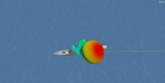
Non-nulled Phased Array Antenna Pattern
Selecting the null direction provider
A phased array antenna not only can steer its maximum gain in a particular direction, but it can also steer nulls toward other directions to prevent radiation to and from other directions. The Phased Array Antenna model's Null Direction Provider enables you to select where the antenna points its nulls. This information is delivered to the beam former, which is responsible for forming and steering the beam toward the specified direction(s).
- Open Ship_Rx's () Properties ().
- Select the Basic - Definition page when the Properties Browser opens.
- Select the Antenna tab.
- Select the Null Direction Provider sub-tab.
- Select the Enabled check box in the Null Steering panel.
- Select LEO_Sat207 () in the available objects list.
- Move () LEO_Sat207 () from the left list to the right list. This is the satellite that is interfering with the ship's communications.
- Click to confirm your changes and to close the Properties Browser.
This tab is within the Model Specs sub-tab, which is itself within the Antenna tab.
The null direction provider selects the pointing directions for nulls based on your selection of STK Objects.
Viewing the nulls
View the effects of your changes on the ship's antenna pattern.
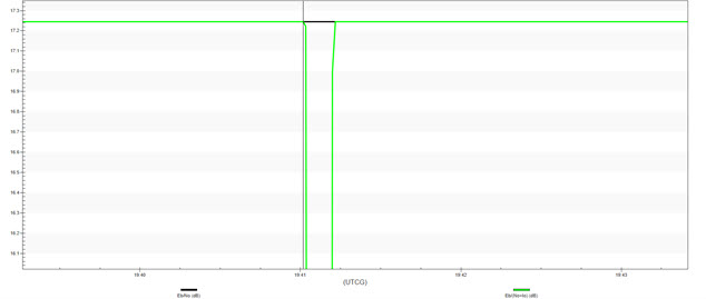
- Bring the EbNo Interference graph to the front.
- Zoom out () on the graph until you can't zoom out any further.
- Click Refresh (F5) (
 ) to refresh the graph.
 - Right click on the lowest spike during the first interference period.
- Select Set Animation Time in the shortcut menu.
- Return to the 3D Graphics window.
- View the nulled antenna pattern.
Note that the first instance of interference has been reduced.
Nulling Effect Shown On Graph
Nulled Antenna Pattern
Saving your work
Save your work and close out of your scenario.
- When you are finished, close the EbNo Interference graph and the Spectrum Analyzer.
- Save () your work.
Summary
This tutorial served as a brief introduction to the Spectrum Analyzer plugin. You began by configuring a maritime VSAT communications link between a ship at sea and a satellite in geosynchronous orbit. You modeled the satellite's transmitter and ship's phased array antenna, then visualized its antenna pattern. Next, you inserted a constellation of Sun-synchronous LEO satellites and their transmitters using the Walker tool. After creating a custom graph of Eb/No and interference, you determined which transmitter was interfering with your communications system using the Spectrum Analyzer plugin. Finally, you adjusted the ship's phased array antenna to incorporate nulls to reduce the interference from the LEO satellite.
On your own
On your own, you can determine which satellite is causing the second interference spike. Use the Spectrum Analyzer to view the interference, and then null the satellite causing the interference.