Part 10:
STK Premium (Air), STK Premium (Space), or STK Enterprise
You can obtain the necessary licenses for this tutorial by contacting AGI Support at support@agi.com or 1-800-924-7244.
Required product install: The Ansys ModelCenter® model-based systems engineering software and the STK Plugin for ModelCenter are required to complete this tutorial.
ModelCenter installation prerequisites: The ModelCenter software requires the installation of a 64-bit version of Java, a 64-bit implementation of Python 3.x, and the installation of the thrift and six Python packages. See the ModelCenter Installation Prerequisites for more information.
This tutorial was written using version 2026 R1 of the Ansys ModelCenter® model-based systems engineering software.
The results of the tutorial may vary depending on the user settings and data enabled (online operations, terrain server, dynamic Earth data, etc.). It is acceptable to have different results.
Capabilities covered
This lesson covers the following capabilities of the Ansys Systems Tool Kit® (STK®) digital mission engineering software:
- STK Pro
- Coverage
- STK Analyzer
Problem statement
Engineers and operators require an easy way to determine how a satellite's orbital parameters, such as its semi-major axis, eccentricity, inclination, argument of perigee, right ascension of the ascending node, and true anomaly, affect the ability a sensor or camera on board to view the surface of the Earth. You want to quickly run multiple trade studies to determine how the inclination, eccentricity, and the combination of both will effect the percentage of coverage over the entire Earth during a 24-hour analysis period.
Solution
Use the STK software's Coverage capability and the Analyzer capability, which is part of the Ansys ModelCenter® model-based systems engineering software, to perform parametric and carpet plot trade studies, which will determine the combination of inclination and eccentricity that provides the highest percentage of global coverage.
What you will learn
Upon completion of this tutorial, you will understand:
- How to wrap an STK scenario with the STK Plugin for ModelCenter
- How to use the Analyzer capability
- How to perform trade studies in the ModelCenter software
Creating a new scenario
First, you must create a new scenario, then build from there.
- Launch the STK application (
 ).
). - Click
 Create a Scenario in the Welcome to STK dialog box.
 - Enter the following in the New Scenario Wizard:
- Click when you finish.
- Click Save (
 ) when the scenario loads. The STK software creates a folder with the same name as your scenario for you.
 - Verify the scenario name and location in the Save As window.
- Click .
| Option | Value |
|---|---|
| Name | STK_ModelCenter |
| Location | Default |
| Start | 8 Jun 2026 16:00:00.000 |
| Stop | 9 Jun 2026 16:00:00.000 |
Save (![]() ) often during this lesson!
) often during this lesson!
Cleaning up your workspace
You can view coverage in both the 2D and 3D Graphics windows. Closing the Timeline View and placing the graphics windows side by side makes this simple to do.
- Close (
 ) the Timeline View at the bottom of the STK application window.
 - Select the Window menu in the Menu Bar.
- Select Tile Vertically.
Your 2D and 3D Graphics windows will fill the available workspace.
Turning off streaming terrain
Analytical and visual terrain is not required in this analysis, so you can turn off
- Open STK_ModelCenter's () Properties (
 ).
). - Select the Basic - Terrain page.
- Clear the Use terrain server for analysis check box in the Terrain Server panel.
- Click to accept your changes and to close the Properties Browser.
Designing an initial orbit
Use the
- Bring the Insert STK Objects Tool (
 ) to the front.
 - Insert a Satellite (
 ) object using the Orbit Wizard (
 ) method.
 - Select the Orbit Designer Type when the Orbit Wizard opens.
- Enter MySat for the Satellite Name.
- Set the following Orbital Elements:
- Click to propagate the satellite and to close the Orbit Wizard.
With the Orbit Designer, you can create any orbit you wish.
| Option | Value |
|---|---|
| Semimajor Axis | 10600 km |
| Eccentricity | 0.363 |
| Inclination | 116 deg |
| Argument of Perigee | 270 deg |
| RAAN | 104 deg |
| True Anomaly | 90 deg |
Attaching a Sensor object to the satellite
Use a
- Insert a Sensor (
 ) object using the Define Properties () method.
 - Select MySat () in the Select Object dialog box.
- Click to confirm your selection and to close the Select Object dialog box.
- Note that the default Sensor Type is set to Simple Conic when the Properties Browser opens.
- Set the Cone Half Angle to 10 deg.
- Click to accept your change and to close the Properties Browser.
- Rename Sensor1 () Camera_View.
A Simple Conic sensor pattern is defined by a simple cone angle, measured in terms of the cone half angle.
MySat in orbit
Using the Coverage capability
The STK software's Coverage capability allows you to analyze the global or regional coverage provided by one or more assets while considering all available accesses. To address area coverage, the Coverage capability provides you with two STK object classes: Coverage Definition objects and Figure of Merit objects.
Inserting a Coverage Definition object
You want to assess coverage over the entire globe. To do this, you will use a
- Insert a Coverage Definition (
 ) object using the Insert Default () method.
 - Rename CoverageDefinition1 () Global_Grid.
Defining the Coverage Grid Area of Interest
Coverage analyses are based on the accessibility of assets (that is, the objects that provide coverage) to the geographical areas of interest. For analysis purposes, the geographical areas of interest are further refined using regions and points defined by the STK application. Points have specific geographical locations and are used in the computation of asset availability. Regions are closed boundaries that contain sets of points. The combination of the geographical area, the regions within that area, and the points within each region is called the
- Open Global_Grid's () Properties ().
- On the Basic - Grid page, change Grid Area of Interest - Type to Global.
- Click to accept your change and to keep the Properties Browser open.
Selecting the coverage assets
Assign the satellite's camera as your coverage asset.
- Select the Basic - Assets page.
- Expand (
 ) MySat () in the Assets list.
 - Select Camera_View ().
- Click .
- Click to accept your changes and to close the Properties Browser.
Inserting a Figure of Merit object
The STK software enables you to specify the method by which the quality of coverage is measured using a
- Insert a Figure Of Merit (
 ) object using the Insert Default () method.
 - Select Global_Grid () when the Select Object dialog box opens.
- Click .
- Rename FigureOfMerit1 () Simple_Cov.
Computing accesses
The ultimate goal of coverage is to analyze accesses to an area using assigned assets. Compute accesses by opening the
- Right-click on Global_Grid () in the Object Browser.
- Select CoverageDefinition in the shortcut menu.
- Select Compute Accesses in the CoverageDefinition submenu.
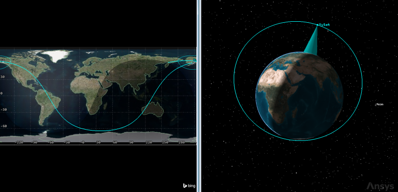
- Bring the 2D Graphics window to the front.
- Review the satellite's areas of coverage across the globe.
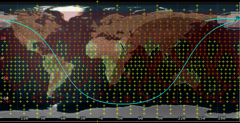
2D Graphics Window Global Coverage
Note that coverage is more complete at higher latitudes.
Creating a Percent Satisfied report
You're interested in the percent of the earth's surface covered as defined by your Simple Coverage definition, meaning the percentage of the coverage grid area covered by at least one asset at some point during the coverage interval. To find this static value, generate a Percent Satisfied report in the Report & Graph Manager. Percent Satisfied reports the percentage of the coverage grid area which is satisfied; it's computed by summing the areas associated with all satisfied grid points, dividing by the total grid area, and multiplying by 100.
- Right-click on Simple_Cov () in the Object Browser.
- Select Report & Graph Manager... (
 ) in the shortcut menu.
 - Select the Percent Satisfied (
 ) report style in the Installed Styles (
 ) folder in the Styles list.
 - Click .
- Note the % Satisfied value at the bottom of the report.
- When finished, close the report and the Report & Graph Manager.
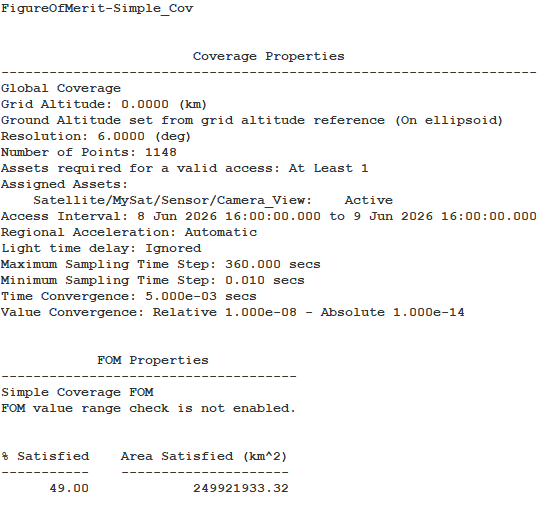
Percent satisfied report
The value you see is the scenario benchmark, which, in this case, is approximately 49 percent.
Closing out of the STK application
With your baseline scenario configured, save your scenario and close out of the STK application in preparation for the next step.
- Save () your scenario.
- Close any open reports, the Report & Graph Manager, and any open tools.
- Close the STK application.
Creating a new ModelCenter project
The
- Open the ModelCenter (
 ) application.
 - Click in the Welcome to ModelCenter dialog box.
- Click when the What type of model would you like to create? dialog box opens.
- Navigate to your scenario folder (for example, C:\Users\<username>\Documents\STK_ODTK 13\STK_ModelCenter.
- Enter STK_ModelCenter in the File name field.
- Ensure the Save as type is set to the ModelCenter Model (Zip) (*.pxcz).
- Click .
Configuring the STK Plugin for ModelCenter
The
- Select favorites (
 ) in the Server Browser at the bottom of the window.
 - Click and drag the STK component (
 ) into the dashed circle underneath "Drop items here to build the model" in your workflow's Analysis View.
 - Select STK_ModelCenter.sc when the Open STK Scenario file dialog box opens.
- Click .
- After a few moments, the STK Analyzer window will open.
The Server Browser resides at the bottom of the ModelCenter window and is used to browse for components that can be used in ModelCenter.
The STK_ModelCenter scenario file will open in the STK application in the background.
Specifying the variables for analysis with Analyzer
Use the STK Analyzer window to configure the input and output variables available for further analysis with the
Selecting the input variables
Your studies will focus on only two of the six orbital elements you set at the beginning of the lesson — inclination and eccentricity. You need to select input and output variables from the main STK Analyzer window to pass to the ModelCenter software's Trade Study tools.
- Select MySat () in the STK Variables tree.
- Expand (
 ) the Propagator (TwoBody) (
 ) property in the STK Property Variables tree.
 - Select Inclination (
 ).
). - Move (
 ) Inclination () to the Analyzer Variables list.
 - Select Eccentricity ().
- Move () Eccentricity () to the Analyzer Variables list.
When you select an object in the STK Variables tree, all possible input variable candidates for that object are listed under the General tab and the Active Constraints tab in the STK Property Variables panel.
Note that both Eccentricity and Inclination are listed as Inputs in the Analyzer Variables list.
Selecting the output variable
The same data providers that are available in the Report & Graph Manager are available in the Data Provider Variables tree. Select Percent Satisfied as the Output variable.
- Expand () Global_Grid () in the STK Variables tree.
- Select Simple_Cov ().
- Expand () the Static Satisfaction (
 ) data provider.
 - Select the Percent Satisfied (
 ) data provider element.
 - Move () Percent Satisfied () into the Analyzer Variables list.
- Click to confirm your selections and to close the STK Analyzer window.
Note that Percent Satisfied is listed under Outputs in the Analyzer Variables list.
This will also close the STK application, which had been running in the background.
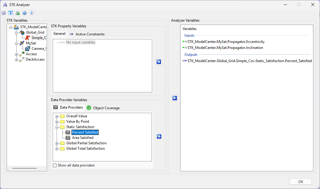
STK Analyzer variables
Determining the impact of satellite inclination on the percentage satisfied
The first study you will perform varies inclination and its effect on global coverage.
Using the Parametric Study tool
The Parametric Study tool runs a workflow through a sweep of values for some input variable. You can plot the resulting data to view trends. Set up a parametric study using inclination as the design variable and percent satisfied as the response.
- Expand () all the elements in the Component Tree.
- Click Parametric Study (
 ) in the Standard toolbar.
 - Click and drag Inclination (
 ) from the Component Tree to the Design Variable field when the Parametric Study tool opens.
 - Set the following Design Variable values:
- Click and drag Percent_Satisfied (
 ) from the Component Tree to the Responses field.
 - Click .
| Option | Value |
|---|---|
| starting value | 112 |
| ending value | 120 |
| step size | 1 |
Design Variable units are not specified in Analyzer. Analyzer assumes the default units set in your STK scenario.
Note the number of samples is automatically set to 9, calculated from the values you set.
Clicking will open the Data Explorer, which is a tool used by Trade Study tools to display data collected from a Model. While data are being collected, the Data Explorer displays a progress meter, a halt button, and the data.
Reviewing the Table page data
The Table page of the Data Explorer displays trade study data in a tabular form. It is the default window that is present for all trade studies. Cells are shaded differently depending on the associated variable's state. Input variables are shown with green text, valid values are displayed with black text, invalid values are displayed with gray text, and modified values are displayed with blue text. From the table it is possible to view and edit all values in your trade study and even to add and remove whole runs.
- Close the 2D Scatter Plot that opened when the trade study finished running.
- Bring the Table page to the front when all runs finish.
- Examine the results in the Data Explorer table.

Inclination Trade Study Table Page
Notice nine runs were performed in one-degree increments from 112 degrees to 120 degrees inclination. Notice the second row shows the global coverage percentage for each change in inclination, and that an inclination of 120 degrees provides the highest percentage of global coverage.
Creating a 2D Line Plot
For this study, you will create a 2D Line Plot. A 2D Line Plot displays an X-Y plot for variables in your model. Any variable in the workflow can be plotted against any other variable.
- Close the 2D Scatter Plot that opened when the trade study finished running.
- Click Add View (
 ) on the Table Page toolbar.
 - Select 2D Line Plot (
 ) in the drop-down list.
Setting options for the axes
Use the Axes tab to set options for the axes.
- Click Axes in the Plot Options menu.
- Select the Ticks tab.
- Change the Max # value to 20.
- Click anywhere on the plot to close the Plot Options menu.
- Review the 2D Line Plot.
The Axes tab is used to set options for the plot's axes.
The Ticks tab is used to set the display of ticks along the axes.
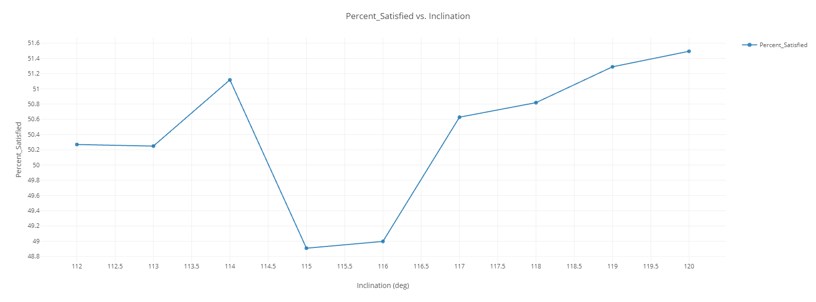
Percent Satisfied vs. Inclination 2D Line Plot
Looking at the 2D Line Plot, you see that inclination of 120 degrees, basing the analysis on one-degree increments, gives you the best choice for global coverage during the 24-hour analysis period.
Closing out your trade study
Close out your trade study to prepare for the next section.
- Close the 2D Line Plot and the Table page when you are finished.
- Click when prompted to close your trade study without saving.
- Leave the Parametric Study tool open.
Studying the satellite's eccentricity
Eccentricity could have an impact on the sensor's footprint. Note that you have to take into consideration the possibility of the satellite colliding with the Earth's surface when changing its eccentricity.
Running a new Parametric Study
Set up a second Parametric Study with eccentricity as the Design Variable and Percent Satisfied as the response.
- Click and drag Eccentricity () from the Component Tree to the Design Variable field when the Parametric Study tool opens.
- Set the following Design Variable values:
- Click .
This will replace Inclination as the Design Variable.
| Option | Value |
|---|---|
| starting value | 0.362 |
| ending value | 0.364 |
| number of samples | 10 |
Creating a 2D Line Plot
Create a 2D Line Plot to investigate the data.
- Close the 2D Scatter Plot that automatically opened after the trade study finished running.
- Click Add View () on the Table Page toolbar.
- Select 2D Line Plot () in the drop-down list.
- Click Axes in the Plot Options menu.
- Select the Ticks tab.
- Change the Max # value to 40.
- Click anywhere on the plot to close the Plot Options menu.
- Hover over one of the design points. The Design Tooltip appears.
The Design Tooltip allows you to quickly examine individual design points.
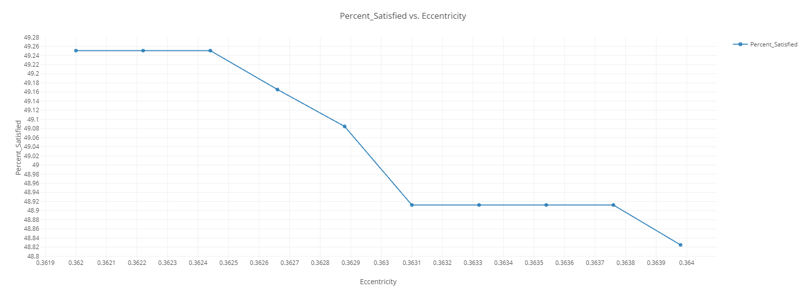
Percent Satisfied Vs. Eccentricity 2D Line Plot
The small change in eccentricity didn't have too much impact on global coverage. 0.362000 through 0.36245 provided a steady value of 49.25 percent satisfied; after that, there is a drop in the satisfaction percentage.
Closing out your trade study
Close out your trade study to prepare for the next section.
- Close the 2D Line Plot and the Table page when you are finished.
- Click when prompted to close your trade study without saving.
- Close the Parametric Study tool.
Using the Carpet Plot tool to study inclination and eccentricity together
A Carpet Plot is a means of displaying data dependent on two variables in a format that makes interpretation easier than normal multiple curve plots. A Carpet Plot can be thought of as a multidimensional Parametric Study. Setting the design variables in a Carpet Plot is similar to using the Parametric Study tool, except you can study two variables simultaneously instead of one.
Creating a new Carpet Plot
Set up a Carpet Plot with inclination and eccentricity as the Design Variables and Percent Satisfied as the response.
- Click Carpet Plot (
 ) on the Analyzer toolbar to access the Carpet Plot tool.
 - Click and drag Inclination () from the Component Tree to the first Design Variables field when the Carpet Plot tool opens.
- Set the following Inclination Design Variable values:
- Click and drag Eccentricity () from the Component Tree the second Design Variables field.
- Set the following Eccentricity Design Variable values:
- Click and drag Percent_Satisfied () from the Component Tree to the Responses field.
- Click .
| Option | Value |
|---|---|
| From | 119 |
| To | 121 |
| Step Size | 1 |
| Option | Value |
|---|---|
| From | 0.361 |
| To | 0.365 |
| Step Size | 0.001 |
Configuring the Carpet Plot's axes
Using the Carpet Plot tool, look for the best combination of inclination and eccentricity. First, make the Carpet Plot easier to read by adjusting its axes, then review the plot.
- Bring the Carpet Plot to the front.
- Click Axes in the Plot Options menu.
- Select the Lines tab.
- Change the Grid Lines value to 10.
- Click anywhere on the plot to close the Plot Options menu.
- Review the plot.
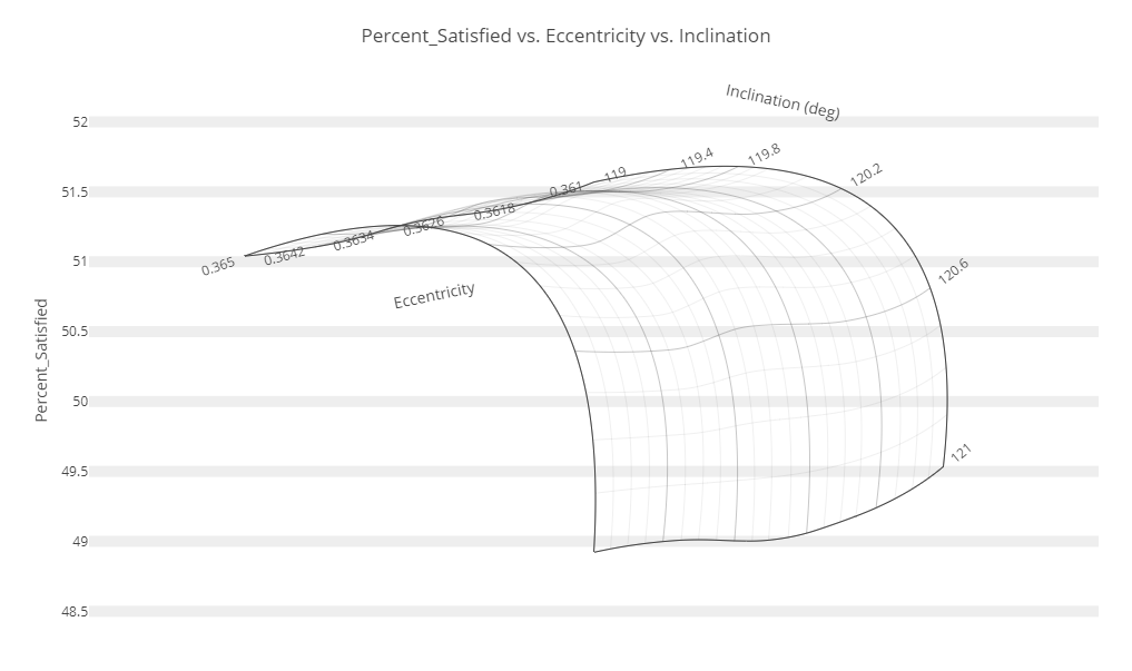
Percent Satisfied vs. Eccentricity vs. Inclination Carpet Plot
The original benchmark of global coverage was approximately 49 percent. In this study, an inclination of 119.6 degrees and an eccentricity of 0.361 provided the best percentage of global coverage of approximately 52 percent.
You can find the exact value for this run in the Data Explorer table.
Running your model
Confirm the data by running your model.
- Close out any open plots, tools, and the Data Explorer window.
- Click when prompted to close your trade study without saving.
- Click on the Value field for Inclination in the Component Tree.
- Enter 119.6.
- Click on the Value field for Eccentricity in the Component Tree.
- Enter 0.361.
- Click Run (
 ) in the Standard Toolbar.
 - Note the progress bar on the STK_ODTK13 component as ModelCenter runs your model.
- When it is complete, note that the value for Percent_Satisfied has been recalculated, and that its icon has changed from to
 , indicating the output is valid.
By running your model, you can see that Percent_Satisfied has been updated to 51.9328, confirming the results from your Carpet Plot Study.
Saving your work
Save your work and close out ModelCenter application.
- Click Save (
 ) to save your ModelCenter workflow.
 - Close the ModelCenter application.
Summary
You began the scenario by placing a Satellite object in a retrograde orbit. You attached a Sensor object to it. The sensor had a 20-degree field of view and was orientated to point straight down below the satellite to the Earth's surface. Using a Coverage Definition object, you created a global coverage grid and assigned the Sensor object as the coverage asset. Using a Figure Of Merit object with a Simple Coverage definition, you determined that approximately 49 percent of the Earth's surface was accessed by them sensor object during a 24-hour analysis period. The satellite's original inclination was 116 degrees and its eccentricity was 0.363. Using the STK Plugin for ModelCenter and the ModelCenter software, you ran two Parametric studies, changing inclination and eccentricity, and studied the effects on global coverage. You ended the analysis by performed a Carpet Plot study, which determined the best combination of inclination and eccentricity that provided the highest percentage of global coverage. Your final value for the inclination was 119.6 degrees and the eccentricity was 0.361. This combination raised global coverage percentage from the benchmark of approximately 49 percent to approximately 52 percent.
On your own
You could rerun all the Parametric studies using new values with the existing input variables. You could add new inputs such as the semi-major axis, and study how that affects coverage. A different approach might be to add an input variable that changes the cone half angle of the Sensor object. There are a lot of combinations you could try.