STK Pro, STK Premium (Air), STK Premium (Space), or STK Enterprise
You can obtain the necessary licenses for this training by contacting AGI Support at support@agi.com or 1-800-924-7244.
This lesson requires STK 12.9 or newer to complete it in its entirety.
The results of the tutorial may vary depending on the user settings and data enabled (online operations, terrain server, dynamic Earth data, etc.). It is acceptable to have different results.
Capabilities covered
This lesson covers the following capabilities of the Ansys Systems Tool Kit® (STK®) digital mission engineering software:
- STK Pro
- Attitude Coverage
Problem statement
A ship in the Western Pacific Ocean is equipped with an onboard sensor that needs to maintain access to as many GPS satellites as possible. The sensor needs to keep a boresight of ten degrees or more from the Sun to avoid performance degradation. You need to analyze GPS satellite coverage in various directions over a 24-hour analysis period to determine which direction is best to point the sensor.
Solution
Use the STK software's Attitude Coverage capability to determine the best direction to point the sensor by identifying the direction that tracks the highest minimum amount of satellites. That direction ensures you will track the most satellites during your 24-hour analysis period. Constrain the sensor to avoid the sun by at least ten degrees, which ensures it will not interfere with the sensor during the analysis period. Finally, use an attitude sphere centered on the ship and an attitude-dependent figure of merit to visualize the attitude coverage regions for situational awareness.
What you will learn
Upon completion of this tutorial, you will have a basic understanding of the following:
- The attitude sphere
- Solar exclusion angles
- Attitude Coverage objects
- Altitude Coverage Figures of Merit
Video guidance
Watch the following video. Then follow the steps below, which incorporate the systems and missions you work on (sample inputs provided).
Creating a new scenario
First, you must create a new STK Scenario and then build from there.
- Launch the STK application (
 ).
). - Click the Create a Scenario (
 ) in the Welcome to STK dialog box.
 - Enter the following in the STK: New Scenario Wizard:
- Click when you finish.
- Click Save (
 ) when the scenario loads. STK creates a folder with the same name as your scenario for you.
 - Verify the scenario name and location in the Save As dialog box.
- Click .
| Option | Value |
|---|---|
| Name | Attitude_Cov |
| Location | Default |
| Start | 1 Oct 2025 07:00:00.000 UTCG |
| Stop | + 24 hrs |
Save (![]() ) often during this lesson!
) often during this lesson!
Turning off streaming terrain
You will not use streaming terrain in this analysis, so you can turn off the Terrain Server.
- Right-click on Attitude_Cov () in the Object Browser.
- Select Properties (
 ).
). - Select the Basic - Terrain page.
- Clear the Use terrain server for analysis check box.
- Click to confirm your change and to close the Properties Browser.
Inserting a Ship object
A
- Bring the Insert STK Objects tool (
 ) to the front.
 - Select Ship (
 ) in the Select An Object To Be Inserted list.
 - Select Insert Default () in the Select A Method list.
- Click
- Right-click on Ship1 () in the Object Browser.
- Select Rename in the shortcut menu.
- Rename Ship1 () Test_Ship.
Setting the ship's route
You can add a route to your ship so it moves as it interacts with the other objects in the scenario.
- Right-click on Test_Ship () in the Object Browser.
- Select Properties () in the shortcut menu.
- Select the Basic - Route page.
- Note the default propagator is GreatArc.
- Set the Reference to WGS84 in the Altitude Reference panel.
- Click twice to add two separate route waypoints.
- Set the following options for waypoints one and two:
- Click to confirm your change and to keep the Properties Browser open.
Since you turned off streaming terrain, WGS84 is the central body's reference ellipsoid.
| Latitude | Longitude |
|---|---|
| 19.00 deg | 125.00 deg |
| 12.00 deg | 140.00 deg |
Adding an altitude sphere
An attitude sphere is a visual aid that you can add to the 3D Graphics and 3D Attitude Graphics windows. When combined with vector displays, the attitude sphere makes a powerful tool for displaying the object's attitude and for tracking attitude changes over time. You need to orient the attitude sphere so that zero (0) degrees longitude matches the ship's direction of travel. This can help later on when orienting the sensor to track the GPS satellites.
- Select the 3D Graphics - Attitude Sphere page.
- Select the Show check box in the Attitude Sphere panel.
- Set the Value to 2.0 in the Scale panel.
- Click next to the Frame field to choose a coordinate frame for the attitude sphere.
- Select Body (
 ) in the Axes For: Test_Ship list when the Select Reference Axes dialog box opens.
 - Click to confirm your change and to close the Select Reference Axes dialog box.
- Click .
Adding a Sun vector
A Sun vector is useful in visualizing that a sensor attached to the ship that avoids the sun by at least ten degrees.
- Select the 3D Graphics - Vector page.
- Select the Sun Vector - Show check box in the Vectors tab.
- Locate the Common Options - Component Size panel.
- Enter 2.0 in the Scale field in the Component Size panel.
- Click .
Viewing the attitude sphere in the 3D Graphics window
View your attitude sphere in the 3D Graphics window.
- Bring the 3D Graphics window to the front.
- Right-click on Test_Ship () in the Object Browser.
- Select Zoom To in the shortcut menu.
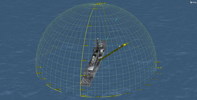
Attitude Sphere
Attaching a sensor to the ship
A Sensor object models the field of view and other properties of a sensing device attached to another STK object.
Inserting a new Sensor object
Attach a sensor object to Test_Ship.
- Bring the Insert STK Objects tool () to the front.
- Insert a Sensor (
 ) object using the Insert Default () method.
 - Select Test_Ship () in the Select Object dialog box.
- Click .
- Rename Sensor1 () Sensor_FOV.
Setting the sensor's field of view
A Simple Conic sensor pattern is defined by a simple cone angle. To define the simple cone, enter the Cone Half Angle.
- Open Sensor_FOV's () Properties ().
- Select the Basic - Definition page.
- Enter 90 deg in the Cone Half Angle field in the Simple Conic panel.
- Click .
Setting the translucency of the sensor projection
Translucency can be adjusted from 0 to 100 percent, where 100 percent is completely invisible.
- Select the 3D Graphics - Attributes page.
- Enter 100 in the % Translucency field in the Projection panel. This is done to avoid the sensor cone in the 3D Graphics window, which would interfere with the display of the attitude sphere.
- Click .
Adding a Sun constraint to the sensor
Sun constraints enable you to impose constraints based on the position of the Sun and Moon.
- Select the Constraints - Active page.
- Click Add new constraints (
 ) in the Active Constraints toolbar.
 - Select Boresight - Solar Exclusion Angle in the Constraint Name list when the Select Constraints to Add dialog box opens.
- Click .
- Click to close the Select Constraints to Add dialog box.
- Use the default Solar Exclusion Angle of 10 degrees.
- Click .
This ensures that Sensor_FOV will ignore access to another object if it is within ten degrees of the Sun.
Propagating the GPS satellites
Insert GPS satellites from the GPS Almanac. You can insert Satellite objects using orbital elements from GPS almanac files. The GPS Almanac is a set of data that every GPS satellite transmits, and it includes information about the state (health) of the entire GPS satellite constellation and coarse data on every satellite's orbit. You can insert an entire GPS constellation with one action by using the
- Bring the Insert STK Objects tool () to the front.
- Insert a Satellite (
 ) object using the Load GPS Constellation (
 ) method.
Note that 31 separate GPS satellites and a Constellation object, GPSConstellation, have been loaded into your scenario.
Using the Attitude Coverage capability
The STK software's
Adding the Attitude Coverage and Attitude Figure Of Merit objects to the Insert STK Objects tool
You can specify which objects appear in the Insert STK Objects tool. Some objects are not listed by default. Ensure that both the Attitude Coverage and Attitude Figure of Merit objects are available in the Insert STK Objects tool by editing the tool's preferences.
- Bring the Insert STK Objects tool () to the front.
- Click .
- Select the Attitude Coverage check box in the Define Default Creation Methods panel when the Preferences dialog box opens.
- Select the Attitude Figure Of Merit check box.
- Click .
Inserting a new Attitude Coverage object
An
- Insert an Attitude Coverage (
 ) object using the Insert Default () method.
 - Select Test_Ship () in the Select Object dialog box.
- Click .
- Rename AttitudeCoverage1 () Sat_Cov.
Setting the point definition properties
In contrast to point definition in the STK Coverage capability, here you are defining the object pointing properties , which depend on the directions represented by points on the
The basic properties of that object (such as a sensor's field of view), including its position at each time step in the coverage interval and any constraints imposed on it, determines the access to the selected assets. These properties are also taken into account in Figure of Merit computations.
- Open Sat_Cov's () Properties ().
- Select the Basic - Grid page.
- Set the following options in the Grid Area of Interest panel:
| Option | Value |
|---|---|
| Type | Latitude Bounds |
| Min. Latitude | 5 deg |
| Max. Latitude | 90 deg |
The Latitude Bounds option tells the STK application to create a grid between user-specified minimum and maximum horizontal boundaries. When the sphere is centered on an Earth-based object, you can use this option to exclude downward directions from consideration or to impose a minimum and maximum elevation angle constraint. In this case, you are only concerned when a satellite is 5 degrees above the horizon to 90 degrees above the ship.
Setting the point granularity
Control the resolution of your coverage analysis by specifying the angular distance between grid points in terms of degrees of latitude and longitude on the sphere. A finer resolution leads to more accurate results, but increases computation time. The STK application stretches grid points in longitude at high and low latitudes in an attempt to preserve the angular area associated with the grid point.
- Enter 10 deg in the Lat/Lon field in the Point Granularity panel.
- Click .
Changing the attitude sphere's 3D Graphics attributes
You can control the display of the attitude coverage grid in the 3D Graphics windows. Make the grid points easier to view in the 3D Graphics window by updating the attitude grid's
- Select the 3D Graphics - Attributes page.
- Change the Color to yellow in the Static Graphics panel.
- Set the Point Size to 4.
- Click .
If you were doing this operationally, you would probably require a grid with more points. For the purposes of this lesson, the grid contains fewer points to keep the calculation time down.
Viewing the attitude coverage grid
View the Attitude Coverage grid in the 3D Graphics window.
- Bring the 3D Graphics window to the front.
- Mouse around in the 3D Graphics window to view the Attitude Coverage grid.
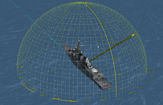
Grid Points
You can see the grid spans from 5 degrees to 90 degrees latitude every 10 degrees.
Adding grid constraints
Sensor_FOV has a 10-degree Solar Exclusion Angle constraint which needs to be applied to the grid.
- Return to Sat_Cov's () Properties ().
- Select the Basic - Grid page.
- Click in the Grid Definition panel.
- Select the Use Object Instance for Constraints check box in the Grid Point Access Options panel.
- Ensure Object Class shows Sensor.
- Select Test_Ship/Sensor_FOV
- Click .
- Click .
Specifying the coverage assets
You can use the Assets properties page to specify the STK objects used to provide coverage. In this case, your assets are the entire constellation of GPS satellites.
- Select the Basic - Assets page.
- Select GPSConstellation (
 ) in the Assets list.
 - Click .
- Click .
Using the Compute Accesses tool
Your can use coverage to analyze accesses to an area with assigned assets and apply necessary limitations upon those accesses. The Compute Accesses tool enables you to compute accesses between the grid points and the assigned assets.
- Select Sat_Cov () in the Object Browser.
- Open the AttitudeCoverage menu.
- Select Compute Accesses.
Adding an Attitude Figure Of Merit object
Determine the best direction in which to point the sensor in order to maximize access from the sensor to the satellites in the constellation. Add an
- Insert an Attitude Figure Of Merit (
 ) object using the Insert Default () method.
 - Select Sat_Cov () in the Select Object dialog box.
- Click .
- Rename AttitudeFigureOfMerit1 () NAsset.
Measuring the number of assets
N Asset Coverage measures the number of assets available simultaneously during coverage, where N is between zero and the total number of assets defined in the coverage definition. You want to examine the lowest number of satellites that you can track by pointing the sensor at various locations. By selecting the location with the highest minimum, you can maximize tracking of the satellites.
- Open NAsset's () Properties ().
- Select the Basic - Definition page.
- Set the following in the Definition panel:
- Click .
| Option | Value |
|---|---|
| Type | N Asset Coverage |
| Compute | Minimum |
Generating a Grid Stats report
Generate a Grid Stats report to determine the highest minimum value. Use this number to create a graphical display of the results in the Attitude Sphere that you can visualize in the 3D Graphics window.
- Right-click on NAsset () in the Object Browser.
- Select Report & Graph Manager... (
 ) in the shortcut menu.
 - Select the Grid Stats (
 ) report in the Installed Styles (
 ) folder when the Report & Graph Manager opens.
 - Click .
- Scroll to the bottom of the report and note the Maximum value (for example, 9 or 10).
- Close the Grid Stats report and the Report & Graph Manager.
Displaying coverage contours
You can display coverage contours on the attitude sphere for Attitude Coverage just as you can on the map and globe for traditional coverage.
- Return to NAsset's () Properties ().
- Select the 3D Graphics - Animation page.
- Clear the Show Animation Graphics check box.
- Click .
- Select the 3D Graphics - Static page.
- Enter 30 in the % Translucency field.
Showing contours
You can specify how levels of coverage quality are displayed in both the 2D and 3D Graphics windows.
- Select the Show Contours option in the Display Metric panel.
- Set the following options in the Level Adding panel, using the minimum and maximum value from your Grid Stats report:
- Click .
- Set the following options in the Level Attributes panel:
- Click .
- Click
- Click to close NAsset's () Properties ().
| Option | Value |
|---|---|
| Start | 0 |
| Stop | 9 or 10 |
| Step | 1 |
| Option | Value |
|---|---|
| Color Method | Color Ramp |
| Start Color | Red |
| End Color | Blue |
Viewing the contours in the 3D Graphics window
You can view the contours in the 3D Graphics window.
- Bring the 3D Graphics window to the front.
- Expand the Static Legend for NAsset dialog box so you can see all the values.
- Use the mouse to zoom out until you can see the entire Attitude Sphere.
- Move the Static Legend for NAsset legend box so that you can see the attitude sphere.
- Close the Static Legend for NAsset dialog box when you are finished.
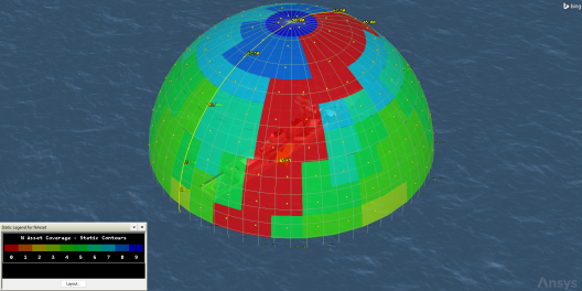
FOM CONTOURS
The blue areas have the highest level of minimum coverage. The path in red shows a coverage level of zero (0). No GPS satellites will be visible to the sensor in the red zone. If you animate the scenario, you can see the sun vector trace a path right through most of the red swath.
You have determined where the most ideal locations would be to aim your sensor boresight under nominal circumstances in order to maximize your tracking of the satellites.
Summary
You inserted into the scenario a Ship object cruising in the Western Pacific Ocean. You enabled an attitude sphere around the ship and aligned the sphere using the ship's body axis. Then, you turned on a sun vector inside the attitude sphere.
You inserted a Sensor object into the scenario and set its field of view to mimic what the ship's pointing sensor can see. You set the boresight solar exclusion angle to ten (10) degrees. The Sensor object won't report any accesses in this area.
Using the Insert STK Objects Tool, you inserted operational GPS satellites into the scenario and automatically grouped them into a Constellation object. Next you inserted an Attitude Coverage object and set the coverage using latitude bounds from 5 to 90 degrees latitude. You constrained the coverage to the sensor's field of view, and used the GPS satellites as your assets.
After computing coverage, you inserted an Attitude Figure of Merit object and set it to use Number of Asset Coverage and computed Minimum. This allowed you to determine the maximum minimum number of satellites your sensor would see when pointing it at various locations in the coverage grid.
Next, you used a Grid Stats report to determine your minimum and maximum values. Using static graphics, you used the minimum and maximum values to visualize colors inside the attitude sphere, which allowed you to determine in which direction to point your sensor to maximize tracking of all the satellites.
Saving your work
Clean up your workspace and close out your scenario.
- Close any open windows except for the 2D and 3D Graphics windows.
- Save () your work.
- Close the scenario when finished.
On your own
Throughout the tutorial, hyperlinks were provided that pointed to in depth information of various subjects. Now's a good time to go back through this tutorial and view that information.