Using Analyzer to Optimize a Satellite Orbit
STK Premium (Air), STK Premium (Space), or STK Enterprise
You can obtain the necessary licenses for this tutorial by contacting AGI Support at support@agi.com or 1-800-924-7244.
This lesson requires version 12.9 of the STK software or newer to complete in its entirety. If you have an earlier version of STK, you can complete a legacy version of this lesson.
Required product install: A 64-bit version of Java is required to run Analyzer. See the Analyzer system requirements for more information.
The results of the tutorial may vary depending on the user settings and data enabled (online operations, terrain server, dynamic Earth data, etc.). It is acceptable to have different results.
Capabilities covered
This lesson covers the following capabilities:
- STK Pro
- Coverage
- STK Analyzer
Problem
Engineers and operators require a quick way to determine how various orbital parameters will affect the ability of a sensor or camera to view the surface of the Earth. Your team wants to launch a satellite into orbit that will be used to monitor icebergs over the polar cap. You will use a low-Earth orbit (LEO) satellite to scan the Earth's surface. Data will then be relayed through a GEO satellite back to a ground processing facility in Montreal. Your purpose is to better understand the requirements for the LEO satellite to include specifying orbit parameters for the satellite and configuration of the sensor.
Solution
To better understand how the LEO satellite orbit and sensor parameters impact coverage capabilities, you will run a series of parametric studies. For each parametric study, you will run a single design parameter through a sweep of values. At each value, you'll collect coverage statistics using a Figure of Merit object. Your solution for this problem is to optimally configure the satellite’s orbit and sensor to best cover the polar ice cap. To initiate your analysis, you will perform a few trade studies to see how changing parameters impacts your coverage capability. This will be followed by creation of a carpet plot to view how multiple parameters impact coverage. Lastly, you'll perform an optimization study to scan through the design space to find a solution that meets your requirements.
What you will learn
Upon completion of this tutorial, you will understand how to:
- Parametrically explore the STK design space in order to optimize your mission
- Perform parameter studies that vary an input variable through a range of values
- Plot one or more output variables
- Analyze an STK scenario for trends
- Generate 3D surface plots and perform optimization studies
- Optimize scenario parameters to meet mission objectives
Video guidance
Watch the following video. Then follow the steps below, which incorporate the systems and missions you work on (sample inputs provided).
Please note, the video refers to a starter scenario accessed from the STK Data Federate (SDF). This scenario is included with your STK install. Please follow the written steps in this tutorial to open the file.
Using a starter scenario
To speed things up and have you to focus on the portion of this exercise that teaches you Analyzer, a partially created scenario has been provided for you.
Loading the starter scenario
The STK scenario (VDF) used with this tutorial is included with the STK installation. To open the scenario:
- Launch the STK® (
 ) application.
 - Click
 Open a Scenario in the Welcome to STK dialog.
 - Select Installed Scenarios in the navigation pane or browse to <STK install folder>\Data\ExampleScenarios.
Opening the VDF
- Select SensorOpt.vdf.
- Click .
Saving the starter scenario as an SC file
When you open the scenario, the STK application will create a folder with the same name as the scenario in the default user folder (C:\Users\<username>\Documents\STK_ODTK 13, for example). The STK application will not save the scenario automatically. When you choose save a scenario, the STK application will default to saving it in the format in which it originated. Therefore, if you open a VDF, the default save format will be a VDF. The same is true for a scenario file (*.sc). To save the VDF as an SC file, change the file format using the Save As procedure:
- Open the File menu.
- Select Save As....
- Select the STK User folder in the navigation pane when the Save As dialog box opens.
- Select the folder with the same name as the scenario.
- Click .
- Select Scenario Files (*.sc) in the Save as type drop-down list.
- Select the Scenario file in the file browser.
- Click .
- Click in the Confirm Save As Dialog box to overwrite the existing scenario file in the folder and to save your scenario.
A scenario folder with the same name as the VDF was created for you when you opened the VDF in the STK application. This folder contains the temporarily unpacked files from the VDF.
Animating the scenario for situational awareness
Slow your animation down and animate the scenario. You can view the link from Montreal (![]() ) to GEO_Relay(
) to GEO_Relay(![]() ) to LEO (
) to LEO (![]() ) to LEO/Ice_Finder (
) to LEO/Ice_Finder (![]() ).
).
- Click Decrease Time Step (
 ) in the Animation toolbar until Time Step is set at 10:00 sec.
 - Click Start (
 ) to animate the scenario.
 - View the LEO (
 ) scan the polar ice cap.
 - Click Reset (
 ) when finished.
Using the Compute Accesses Tool
The ultimate goal of STK's Coverage capability is to analyze accesses to an area using assigned assets and applying necessary limitations upon those accesses. Compute coverage with the Compute Accesses tool. Arctic_Monitor's (![]() ) grid area of interest is the Area Target (
) grid area of interest is the Area Target (![]() ) named Arctic. Arctic_Monitor's (
) named Arctic. Arctic_Monitor's (![]() ) asset is Relay_Chain (
) asset is Relay_Chain (![]() ).
).
- Right-click Arctic_Monitor (
 ) in the Object Browser.
 - Select CoverageDefinition.
- Select Compute Accesses.
Generating a Grid Stats Report
Your scenario analysis time is seven (7) days. CoveragePerDay's (![]() ) definition is set to Coverage Time and computing Per Day. Per Day is the total coverage time divided by the number of days in the coverage interval. You will use Analyzer to perform trade studies on CoveragePerDay's (
) definition is set to Coverage Time and computing Per Day. Per Day is the total coverage time divided by the number of days in the coverage interval. You will use Analyzer to perform trade studies on CoveragePerDay's (![]() ) Grid Stats report. To understand this report, you'll first manually collect data in STK. Generate a Grid Stats report to see the smallest to largest number of accesses to any point in the grid.
) Grid Stats report. To understand this report, you'll first manually collect data in STK. Generate a Grid Stats report to see the smallest to largest number of accesses to any point in the grid.
- Right-click CoveragePerDay (
 ) in the Object Browser.
 - Select Report & Graph Manager... (
 ).
). - Select the Grid Stats (
 ) report in the Installed Styles (
 ) list.
 - Click .
- Note the Minimum, Maximum, and Average values in the report. These values will be accessible in Analyzer as output variables.
- Close (
 ) the Grid Stats report when finished.
 - Close () the Report & Graph Manager.
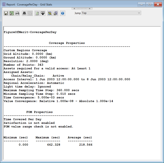
Grid Stats Report
This report indicates that for all the grid points defining the polar cap, at least one point is not seen by the satellite (Minimum = 0), at least one point is seen for ~662 seconds, and on average points are seen for ~219 seconds per day during your analysis period.
Introduction to Analyzer
Analyzer provides a set of analysis tools that:
- Enable you to understand the design space of your systems.
- Enable you to perform analyses in STK easily, without involving programming or scripting.
- Introduce trade study and post-processing capabilities.
- Can be used with all STK scenarios, including those with STK Astrogator satellites.
Configuring Analyzer
Start by opening Analyzer in STK.
- Click View on the STK menu bar.
- Select Toolbars in the drop-down menu.
- Select Analyzer in the next drop-down menu.
- Click Analyzer... (
 ) on the Analyzer toolbar.
Analyzer imports a copy of the currently loaded Scenario. You can add any of the STK variables as Analyzer input or output variables. If you change a value of a variable in your scenario through the STK interface, you should re-add the variable as an Analyzer variable before running any trade studies with the new value.
Selecting satellite input variables
You will start by selecting the satellite orbit variables, such as Inclination, RAAN, and the Semi-major Axis, as input variables.
- Select LEO () in the STK Variables list.
- Expand (
 ) Propagator (J4Perturbation) (
 ) in the STK Property Variables list.
 - Double-click the following STK Property Variables (
 ) to move them to the Analyzer Variables list:
 - SemiMajorAxis
- Inclination
- RAAN
Selecting Figure of Merit output variables
The output variables will be average, minimum, and maximum coverage per day of the Arctic Monitor.
- Expand () Arctic_Monitor () in the STK Variables list.
- Select CoververagePerDay ().
- Expand () Overall Value () in the Data Provider Variables list.
- Double-click the following data provider elements (
 ) to move them to the Analyzer Variables list:
 - Minimum
- Maximum
- Average
Implementing the Parametric Study Tool
The Parametric Study Tool runs a model through a sweep of values for some input variable. You can plot the resulting data to view trends.
- Click Parametric Study... (
 ) on the Analyzer toolbar.
 - View the Parametric Study Tool window.
- Look at the Component Tree on the left. It lists variables that you selected in Analyzer.
- Look at the fields on the right. They are used to specify which variables you should use in the study.
Setting up an inclination Parametric Study
Defining Design Variables
Set up a Parametric Study with Inclination as the design variable.
- Drag and drop Inclination (), the Design Variable, from the Component Tree on the left to the Parametric Study Tool's Design Variable on the right.
- Set the following Design Variable parameters:
| Option | Value |
|---|---|
| starting value | 45 |
| ending value | 135 |
| step size | 10 |
Defining Responses
Set Minimum, Maximum, and Average as the Responses.
- Drag and drop the following data provider elements () into the Responses field:
- Minimum
- Maximum
- Average
- Click
Investigating the Data Explorer
The Data Explorer is a Trade Study tool used to display data collected from STK. While data is being collected in the Table, the Data Explorer window displays a progress meter, a halt button, and the data. Once the Parametric study is complete, the Table page and 2D Scatter Plot display the collected data.
- Bring the Table page to the front when all runs are completed.
- Scroll across the Table to see the results.
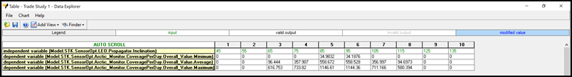
Table Page
Creating a 2D Line Plot
Create a 2D Line Plot from the Table page.
- Click Add View in the Table Page toolbar.
- Select 2D Line Plot in the drop-down menu.
Updating the graph
Update the graph to display each Inclination versus the Maximum, Minimum, and Average coverage time. Maximum will be Series 1, Minimum will be Series 2, and Average will be Series 3.
Creating Series 1
Select Maximum as Series 1.
- Click in the menu on the left.
- Open the y drop-down menu in the Dimensions dialog.
- Select Maximum. This changes Series 1 to Maximum (sec).
Creating Series 2
Select Minimum as Series 2.
- Click Add Series at the top of the Dimensions dialog. This creates Series 2.
- Open the x drop-down menu.
- Select Inclination.
- Open the y drop-down menu.
- Select Minimum. This changes Series 2 to Minimum(sec).
Creating Series 3
Select Average as Series 3.
- Click Add Series at the top of the Dimensions dialog. This creates Series 3.
- Open the x drop-down menu.
- Select Inclination.
- Open the y drop-down menu.
- Select Average. This changes Series 3 to Average(sec).
- Click the graph to exit out of the menu.
Analyzing the 2D line plot
Results from the first study are as expected: the closer the inclination is to 90 degrees, the better your coverage capability will be. This makes sense, as the ice cap covers the North Pole and your coverage will be best when your orbit takes you through the rotational center point of the area you are trying to cover.
There are two additional interesting trends in the data.
- First, maximum coverage does not smoothly improve as inclination approaches 90 degrees.
- Second, and more importantly, the minimum coverage value does not climb above zero until inclination reaches some value between 75 and 90 degrees.
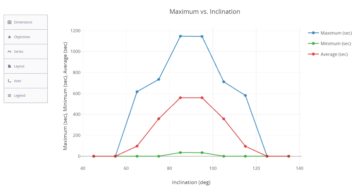
2D Line Plot
Cleaning up your scenario
Before continuing, close some of your windows.
- Bring the Table page to the front.
- Close () the Table page.
- Click when asked to save the study. This will close any graphs associated with the trade study.
Refining the trade study parameters
Since you want to ensure that your orbit will cover the entire ice cap, you want to run a more refined parametric study in the area of interest.
- Return to the Parametric Study () Tool. If you don't see it, it might be located behind the STK Analyzer window.
- Set the following Design Variable parameters:
- Click .
| Option | Value |
|---|---|
| starting value | 85 |
| ending value | 95 |
| step size | 1 |
Understanding Table page data
You can create line plots that are great for presentations or personal choice, but you can also obtain the required information from the Table page.
- Bring the Table page to the front when all runs finish.
- Use your cursor to expand the table of runs so that you can see all eleven (11) runs.
- Close () the Table page.
- Click when asked to save the study.
This study gives us a much better understanding of where to position the satellite to give you the best overall inclination to ensure maximum coverage of the whole ice cap. You can see that inclinations between 87 and 93 degrees will give you at least 2000 seconds of maximum coverage of the ice cap during your analysis period.
Syncing data from the Parametric Study Tool to STK
You can sync data from STK into the Parametric Study Tool or vice versa. You can make changes in the Component Tree and sync the changes back to STK.
- Return to the Parametric Study () Tool.
- Click the Inclination value in the Component Tree.
- Enter the value 90.
- Press the Enter key on your keyboard.
- Click at the bottom of the Component Tree. This sets LEO's () inclination to 90 degrees in STK. It also recomputes coverage.
- Return to the Parametric Study () Tool.
Determining the impact of RAAN on coverage
RAAN (right ascension of the ascending node) might impact your coverage.
- Highlight everything in the Design Variable field.
- Press Backspace on your keyboard. This clears the variable, so that you can enter a new variable.
- Drag and drop RAAN () from the Component Tree to the Design Variable field.
- Set the following Design Variable parameters:
- Click .
| Option | Value |
|---|---|
| starting value | 0 |
| ending value | 360 |
| step size | 30 |
Understanding the Table page data
Investigate the results.
- Bring the Table page to the front when all runs are completed.
- Use your cursor to expand the table of runs so that you can see all thirteen (13) runs.
- Look at the data in the Table page.
- Click Add View in the Table Page toolbar.
- Select 2D Line Plot in the drop-down menu.
- Bring the Table page to the front.
- Close () the Table page.
- Click when asked to save the study.
At first glance, the data appears to be fairly insensitive to RAAN. This may be due to the difference in scales minimum and maximum coverage values. To view just the minimum coverage values, create a new graph.
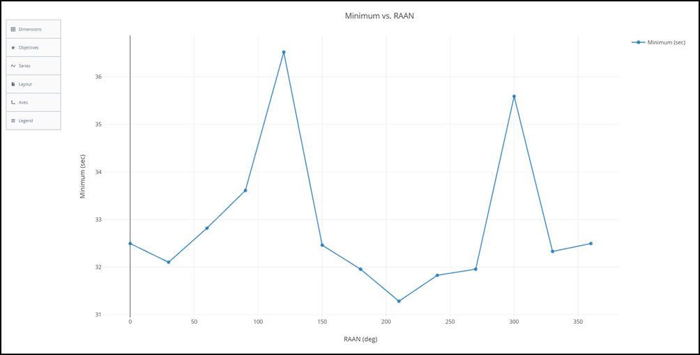
minimum time versus RAAn
Minimum coverage values fluctuate for different RAAN values. This is an artifact of the low frequency sampling of the data. While the difference between high and low values is less than 10 percent of the mean, there are definitely some values that are better than others.
Determining the impacts of altitude on coverage
The final orbit parameter impacting coverage is the altitude of the orbit, the semimajor axis. Vary the orbit from 6,500 to 7,500 kilometers.
- Return to the Parametric Study () Tool.
- Clear RAAN from the Design Variable field.
- Drag and drop SemiMajorAxis () from the Component Tree to the Design Variable field.
- Set the following Design Variable parameters:
- Click .
| Option | Value |
|---|---|
| starting value | 6500 |
| ending value | 7500 |
| step size | 100 |
Understanding Table Page data
Obtain the required information from the Table page.
- Bring the Table page to the front.
- Use your cursor to expand the table of runs so that you can see all eleven (11) runs.
- Close () the Table Page.
- Click when asked to save the study.
There is an interesting trend here. Maximum and average coverages increase rapidly with altitude until a certain altitude is reached, at which point there is an equally sharp drop off. Minimum coverage continues to increase even as maximum and average coverage decreases. This is due to a resolution constraint of 5 meters, as you need to be able to resolve icebergs as small as 5 meters in diameter. Coverage capabilities increase with orbit altitude because the sensor swath also increases. They also decrease beyond a certain altitude because the sensor can no longer resolve 5-meter objects. Your conclusion from this trade study is that your maximum coverage capability is best with a semimajor axis of about 6800 km.
Changing Sensor object resolution
The Sensor (![]() ) object's resolution constraint might have an impact on your trade study. Confirm this by rerunning the study with the Ground Sampling Distance constraint disabled.
) object's resolution constraint might have an impact on your trade study. Confirm this by rerunning the study with the Ground Sampling Distance constraint disabled.
- Bring STK to the front.
- Right-click Ice_Finder (
 ) in the Object Browser.
 - Select Properties ().
- Select the Constraints - Active page.
- Select Ground Sample Distance in the Active Constraints list.
- Clear the Max: check box in the Constraints Properties - Ground Sample Distance frame.
- Click to accept your change and keep the Properties Browser open.
You might need to move or minimize Analyzer and the Parametric Study Tool to the side in order to perform the following tasks.
Rerunning the Parametric Study
Rerun the Parametric Study.
- Bring the Parametric Study () Tool to the front.
- Click .
Understanding Table page data
Obtain the required information from the Table page.
- Bring the Table page to the front.
- Use your cursor to expand the table of runs so that you can see all eleven (11) runs.
- Close () the Table page.
- Click when asked to save the study.
- Close () the Parametric Study () Tool.
The resulting parametric study indicates that without a resolution constraint, as altitude increases, coverage capabilities also increase for all three (3) output variables.
Resetting the Sensor object's resolution constraint
Reset the Sensor (![]() ) object's resolution constraint for further trade studies
) object's resolution constraint for further trade studies
- Bring STK to the front.
- Return to Ice_Finder's () properties ().
- Select the Constraints - Active page.
- Select Ground Sample Distance in the Active Constraints list.
- Select the Max check box in the Constraints Properties - Ground Sample Distance frame.
- Ensure Max is set to 5 m.
- Click to accept your changes and close the Properties Browser.
Using the Carpet Plot tool
A Carpet Plot is a means of displaying data dependent on two variables in a format that makes interpretation easier than normal multiple curve plots. A Carpet Plot can be thought of as a multidimensional Parametric Study.
You have determined that inclination and altitude have significant impacts on coverage capability while the RAAN has minimal influence. Altitude had an increasingly positive impact until the ground sample distance constraint came into effect. Coverage generally improves as inclination approaches 90 degrees. This leads to two questions:
- Does changing altitude impact our conclusions about inclination?
- Can we improve our sensor characteristics to permit a higher altitude orbit?
You will answer the first question by performing a multidimensional Parametric Study (Carpet Plot). You can answer the second question later in the scenario.
Opening the Carpet Plot Tool
Open the Carpet Plot Tool in Analyzer.
- Return to Analyzer.
- Click Carpet Plot... (
 ) in the STK Analyzer toolbar to open the Carpet Plot Tool.
Studying two variables
Set Inclination and SemiMajorAxis as your Design Variables.
- Drag and drop Inclination () from the Component Tree to the first Design Variables field.
- Set the following Inclination Design Variables parameters:
- Drag and drop SemiMajorAxis () from the Component Tree to the second Design Variables field.
- Set the following SemiMajorAxis Design Variables parameters:
| Option | Value |
|---|---|
| From | 85 |
| To | 105 |
| Step Size | 5 |
| Option | Value |
|---|---|
| From | 6500 |
| To | 7500 |
| Step Size | 200 |
Setting the output variables
Set minimum, maximum, and average as the Responses.
- Drag and drop the following data provider elements () into the Responses field.
- Minimum
- Maximum
- Average
- Click .
Be patient. A total of 30 runs are required and this could take a couple of minutes to complete.
Creating a contour plot
Create a Contour Plot from the Table page.
- Bring the Table page to the front when all runs are completed.
- Click Add View.
- Select Contour Plot in the shortcut menu.
Customizing the contour plot
Display Average versus SemiMajorAxis versus Inclination.
- Click in the menu on the left.
- Open the z drop-down menu.
- Select Average.
- Click the graph to exit out of the menu.
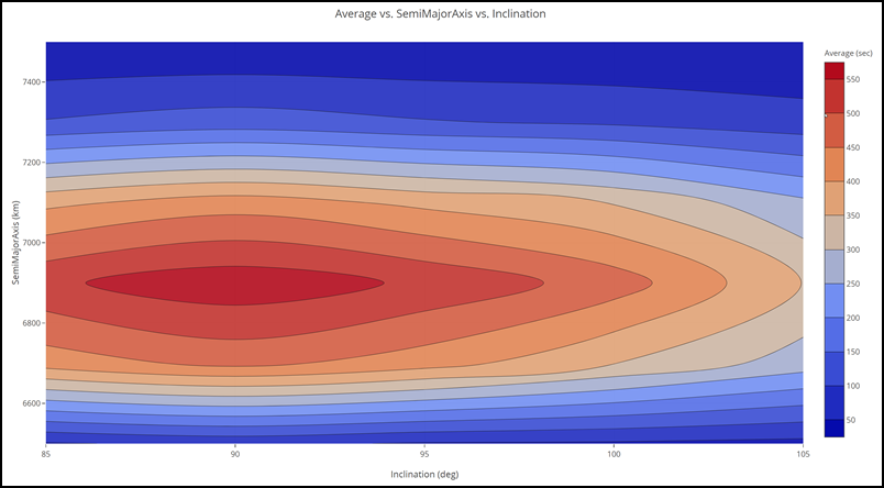
Contour plot
The contour plot indicates that, regardless of altitude, the likely optimal inclination for the best average coverage time is around 90 degrees and the altitude is somewhere between 6800 and 7000 kilometers.
Creating a 3D scatter plot
Create a 3D Scatter Plot.
- Click Add View on the Contour Plot toolbar.
- Select 3D Scatter Plot in the shortcut menu.
Displaying Inclination versus Semi Major Axis versus Average coverage time
Display Inclination vs Semi Major Axis vs Average coverage time.
- Click .
- Open the z drop-down menu.
- Select Average.
- Click the graph to exit out of the menu.
- Bring the Table page to the front.
- Close () the Table page.
- Click when asked to save the study.
- Close () the Carpet Plot Tool.
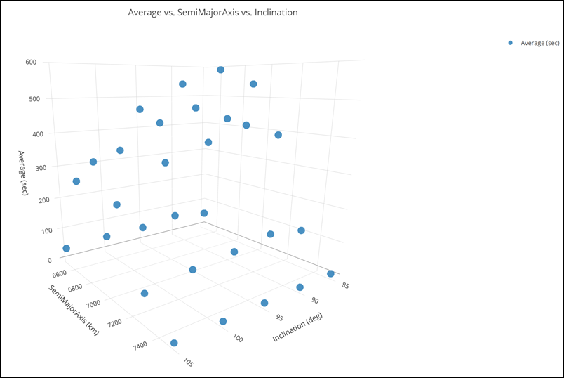
3D Scatter Plot
Studying Sensor object resolution
You now know that for any given inclination, increasing orbit altitude will improve coverage. However, you must take into account the ground sampling resolution constraint for the Sensor (![]() ) object. You can change Ice_Finder's (
) object. You can change Ice_Finder's (![]() ) properties to permit greater viewing capabilities at higher altitudes.
) properties to permit greater viewing capabilities at higher altitudes.
Selecting Sensor input variables
Select your Sensor (![]() ) object input variables.
) object input variables.
- Bring Analyzer to the front.
- Expand () LEO () in the STK Variables list.
- Select Ice_Finder ().
- Expand () SimpleConic () in the STK Property Variables list.
- Double-click coneAngle () to move it to the Analyzer Variables list.
- Expand () Resolution () in the STK Property Variables list.
- Double-click FocalLength (
 ) to move it to the Analyzer Variables list.
 - Double-click DetectorPitch () to move it to the Analyzer Variables list.
Syncing data from the Parametric Study Tool to STK
Set the inclination back to 90 degrees.
- Click Parametric Study... () on the Analyzer toolbar to open the Parametric Study Tool.
- Click the Inclination value in the Component Tree.
- Enter the value 90.
- Press the Enter key on your keyboard.
- Click at the bottom of the Component Tree. This sets LEO's () inclination to 90 degrees in STK.
- Return to the Parametric Study ( ) Tool.
Studying detector pitch
You will focus on maximum coverage for now.
- Drag and drop DetectorPitch () from the Component Tree to the Design Variable field.
- Set the following DetectorPitch Design Variable parameters:
- Drag and drop the Maximum data provider into the Responses field.
- Click .
| Option | Value |
|---|---|
| starting value | .0001 |
| ending value | .001 |
| step size | .0001 |
Creating a 2D Line Plot
Create a 2D Line Plot to investigate the data.
- Bring the Table page to the front when all runs are completed.
- Click Add View on the Table page toolbar.
- Select 2D Line Plot in the drop-down menu.
Customizing the 2D line plot
Customize the graph.
- Click in the menu on the left.
- Select Ticks in the Axes dialog.
- Enter the value 20 in the Max # field.
- Press the Tab key on your keyboard.
- Click the graph to close the Axes dialog.
- Bring the Table page to the front.
- Close () the Table page.
- Click when asked to save the study.
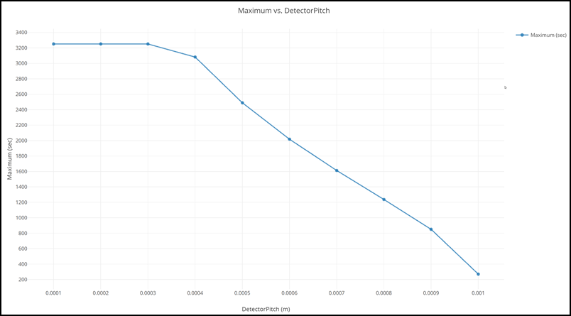
Maximum Seconds vs. Detector Pitch
Detector pitch has a maximum threshold value (.0003 m), which if exceeded will result in degraded coverage capabilities.
Studying Sensor focal length
Determine the impacts of focal length on coverage.
- Return to the Parametric Study Tool.
- Clear DetectorPitch from the Design Variable field.
- Drag and drop FocalLength () from the Component Tree to the Design Variable field.
- Set the following FocalLength Design Variable parameters:
- Click .
| Option | Value |
|---|---|
| starting value | 50 |
| ending value | 200 |
| step size | 10 |
Creating a 2D line plot
Create a 2D line plot to investigate the data.
- Bring the Table page to the front when all runs are completed.
- Click Add View on the Table page toolbar.
- Select 2D Line Plot in the drop-down menu.
Customizing the 2D line plot
Customize the graph.
- Click .
- Select Ticks in the Axes dialog.
- Enter the value 20 in the Max # field.
- Press the Tab key on your keyboard.
- Click the graph to close the Axes dialog.
- Bring the Table Page to the front.
- Close () the Table Page.
- Click when asked to save the study
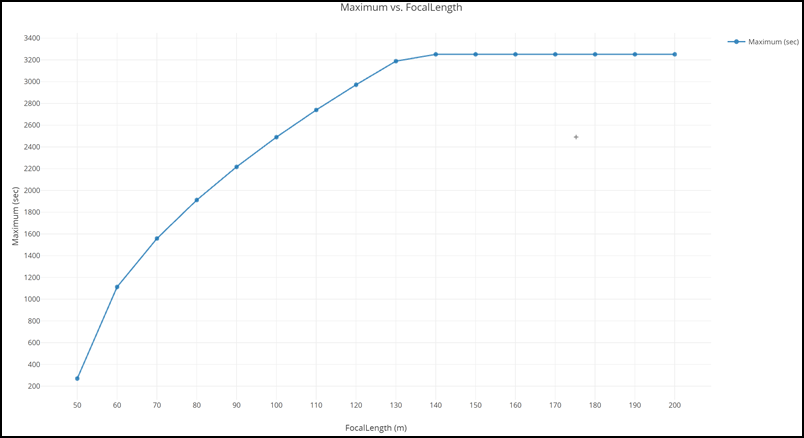
Maximum Seconds vs. Focal Length
Focal length has a threshold value of approximately 140 m. After that, further increases don't improve coverage.
Studying Sensor cone angle
Determine the impact of the cone angle sensor parameter.
- Return to the Parametric Study () Tool.
- Clear FocalLength from the Design Variable field.
- Drag and drop coneAngle () from the Component Tree to the Design Variable field.
- Set the following coneAngle Design Variable parameters:
- Move Maximum from the Component Tree to the Responses list if needed
- Click .
| Option | Value |
|---|---|
| starting value | 20 |
| ending value | 60 |
| step size | 5 |
Creating a 2D line plot
Create a 2D line plot to investigate the data.
- Bring the Table page to the front when all runs are completed.
- Click Add View on the Table page toolbar.
- Select 2D Line Plot in the drop-down menu.
- Bring the Table page to the front.
- Close () the Table page.
- Click when asked to save the study.
- Close () the Parametric Study () Tool.
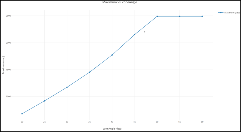
Maximum Seconds vs. Cone Angle
The cone angle has a threshold value of approximately 50 degrees.
Opening the Optimization Tool
Sensor parameters have a large impact on coverage capabilities. To optimize these parameters, you can either guess at values or employ an Optimization Tool. Although you can see trends from the previous studies, guessing at values will be difficult because you are dealing with multiple parameters at the same time and the trends, thus far, assume only one or two parameters are changed at a time.
To solve more complex problems, an optimization tool can be a very useful. An optimizer is an automated tool that makes mathematical calculations about a design problem and incrementally attempts to find an optimal solution. You will use the optimizer to minimize the focal length requirement for the sensor while maintaining a minimum coverage capability of 150 seconds per day for your coverage area.
- Bring Analyzer to the front.
- Click Optimization Tool... (
 ) on the Analyzer toolbar to open the Optimization Tool.
 - Click the inclination value in the Component Tree.
- Enter the value 90.
- Press the Enter key on your keyboard.
- Click .
Creating an objective
The objective functions can be specific variables or equations composed of multiple output variables.
- Drag and drop FocalLength () from the Component Tree to the Objective list in the Objective Definition frame.
- Check that the Value is 100.
- Ensure the Goal is set to minimize.
Selecting the constraints
Constraints restrict particular variables to a region or value.
- Drag and drop Minimum from the Component Tree to the Constraint list.
- Click twice in the cell below Lower Bound.
- Enter the value 150.
- Press the Tab key on your keyboard. There is no upper bound.
Selecting the Design Variables
The design variables are the variables that the optimizer will modify to meet the objective. You want the optimizer to minimize the FocalLength by changing coneAngle, FocalLength, and DetectorPitch.
Selecting coneAngle
- Drag and drop coneAngle () from the Component Tree to the Design Variable list in the Design Variables frame.
- Set the following coneAngle Design Variable parameters:
| Option | Value |
|---|---|
| Lower Bound | 20 |
| Upper Bound | 60 |
Selecting FocalLength
- Drag and drop FocalLenth () from the Component Tree to the Design Variable list.
- Set the following FocalLenth Design Variable parameters:
| Option | Value |
|---|---|
| Lower Bound | 50 |
| Upper Bound | 200 |
Selecting DetectorPitch
- Drag and drop DetectorPitch () from the Component Tree to the Design Variable list.
- Set the following DetectorPitch Design Variable parameters:
| Option | Value |
|---|---|
| Lower Bound | .0001 |
| Upper Bound | .001 |
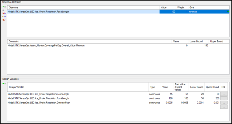
optimization tool values
Using the Darwin algorithm
You will use the Darwin algorithm, which is an advanced optimization algorithm that was developed to efficiently solve difficult real-world design problems.
- Return to the Optimization Tool ().
- Select Darwin in the Algorithm drop-down menu.
- Click .
Be patient. This will take a while to complete.
Investigating Optimization Tool output
You are interested in the best design values.
- Return to the Optimization Tool () when all runs are completed.
- Click .
- Select the Best Design tab when the Optimization Tool Results dialog opens.
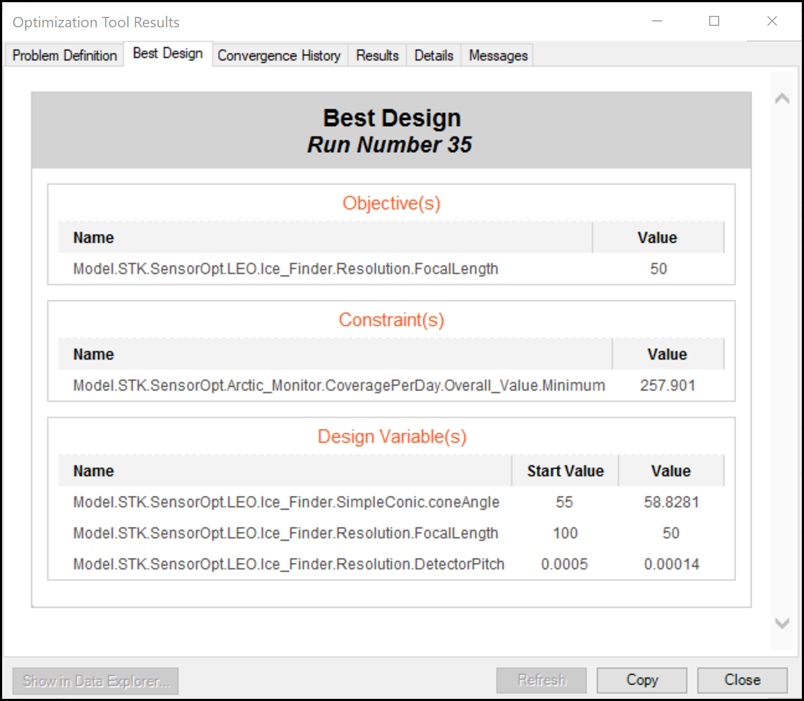
optimization tool Best design values: example only
Your image results for data values and best design run may be different from the above image. A different algorithm was used to generate this example.
After running an optimization study, the values in your scenario will be changed to the final, optimized values. They will not be changed back to what they were before starting the study.
Cleaning up your scenario
Close any open tools and windows to clean up your scenario.
- Click to close the Optimization Tool Results dialog box.
- Bring the Table page to the front.
- Close () the Table page.
- Click when asked to save the study.
- Close () the Optimization Tool ().
- Click to save as a favorite.
- Close () STK Analyzer.
Saving your work
Always remember to save your scenario!
- Return to STK.
- Save (
 ) your work.
Summary
You wanted to understand how a LEO satellite orbit and sensor parameters impact coverage capabilities. Your solution for this problem was to optimally configure the satellite’s orbit and sensor to best cover the polar ice cap. You did this by running a series of parametric studies. For each parametric study, you analyzed a single design parameter through a sweep of values. You collected coverage statistics using a Figure of Merit. Next you created a carpet plot to view how multiple parameters impact coverage. You used the optimization tool to scan through the design space to find a final solution that met your requirements.