EOIR Sensor Properties

STK's EOIR capability supports up to 24 sensors and up to 36 bands per sensor. Bands share a common location and line of sight, but otherwise can have different parameters. Two typical uses for bands are to simulate:

• Different wavelength response capabilities, as for multiband sensor
• Different image magnifications, as for different settings of a zoom lens

To define an EOIR sensor, go to the Definition page of the Sensor properties and select EOIR as the Sensor Type.

For an example of how to use EOIR and STK to measure the visual magnitude of stars, see Shining a Light on Visual Magnitude (PDF).

Adding bands

At the top of the properties Definition page is a list of the bands for the EOIR sensor. Click Add to add a new band for an EOIR sensor and enter its name in the Band Name text box. To delete a band, select it in the list and click Remove. You can also select whether or not to render each band by selecting the Render Band check box next to the band name.

Defining bands

You can define the following types of properties for each band in an EOIR sensor:

• Spatial
• Spectral
• Optical
• Radiometric

To view or modify the properties for a particular band, select it in the list of bands and select one of these four properties tabs. The spatial, spectral, optical, and radiometric properties panels display the values of the highlighted band. For descriptions of the parameters under each of these tabs, click the links above.

Sensor-level properties

You can also define certain properties that apply to the EOIR sensor in general, including all bands. These properties all appear below the band-specific tabs on the Definition panel. For details on specifying sensor jitter, see Jitter. The following table describes the other properties.

Property	Description
Processing Level	From the following list, select the type of calculation performed by this EOIR Sensor-Scene Generator pair: Sensor Off. EOIR does not perform processing for the sensor. Geometric Input. EOIR only calculates and displays the geometric information in the sensor scene. Relative shading of objects is based on the temperature of their thermal models. This selection is helpful for more rapidly stepping through a series of scenes (through time) until arriving at a scene of interest or creating a temperature map. Radiometric Input. EOIR generates a full sensor scene, including both geometric and radiometric aspects. However, it does not apply optical or detector effects. This output is often called entrance aperture radiance. Sensor Output. The EOIR sensor model operates on the sensor scene and calculates the corresponding sensor output image. Each of these successive modes is more computationally intensive and will require more time to generate an image.
Scan Mode	EOIR uses 2D Framing Array as the type of scan mode for processing-level calculation. You cannot modify this.
Show Motion Blur	During the integration time, both the sensor and the objects in the scene are potentially moving. By selecting this check box, EOIR will simulate motion blur as follows: For area targets, it will simulate the gross sensor rotation during the integration time period. For point sources, it will simulate their straight line of motion from their relative sensor position from the start of the integration time to the current scenario time.
Smear Rate	Enter values in mrad/sec for the along-scan and across-scan smear rate of the EOIR sensor relative to the sensor up vector.

Jitter

You can model sensor jitter by either applying Gaussian line-of-sight motion or by using a jitter file.

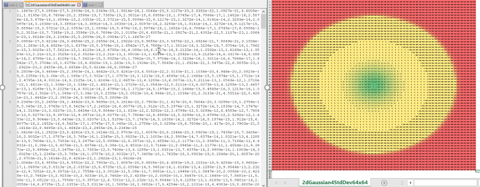
A jitter file is a two-dimentional matrix of CSVs that gives certain values related to the light coming down the center beam that would land on the image plane. In the illustration, the values on the left correspond to the first six rows of dots across the top of the diagram on the right. This particular diagram represents a typical probability distribution, where the probabilities are very low at the edges (red) and rise sharply when approaching the center (green).

In the Jitter subpanel, you can select the following jitter modeling parameters:

Parameter	Description
(method)	Using the shortcut menu, select one of the following modeling methods for assigning jitter values: LOS Gaussian tells EOIR to apply a Gaussian probability distribution about the center beam. You must also specify a value for Line of Sight Jitter, described below. See the diagram after this table. PSF/Realization Filespecifies the probability distribution as a point spread function. The sum of all the values should total 1.0. MTF Filespecifies a frequency modulation transfer function distribution, which is the same as PSF/Realization but in the frequency spectrum. The values are complex numbers that represent the amplitude (real part) and the phase shift (imaginary part). Power Spectrum Fileis the MTF squared, so values don't have an imaginary part.
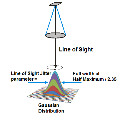
Line of Sight Jitter	Vibrations of a sensor's parent object can cause the Line of Sight to move during integration time, blurring the image. Enter an angle that describes the dimension of an assumed Gaussian motion of the Line of Sight, and EOIR will interpret it as (Full Width at Half Maximum)/2.35. This parameter is only valid for LOS Gaussian type.
Data File	Click the ellipsis to browse to and select a jitter file. The file can be your own or one included in the STK install, typically in <STK install>/EOIR_Databases/PropertyFiles/Shape_Files. This parameter is not available for LOS Gaussian method.
Data File Sampling	Enter a value for one of the following two sampling settings: a spatial sampling value in mrad; for PSF/Realization type only a sampling frequency in cycles/mrad; for MTF and Power Spectrum types

The following is a diagram of the LOS Gaussian method modeling.

You can create a Windows user environment variable to speed up and improve EOIR image fidelity. The user environment variable AGI_EOIR_SENSOR_OSF can have the values 1, 2, 4, 8, 16, and 32. Each of these specifies how EOIR sensors will oversample spatial data, resulting in differences in both performance and fidelity. A lower value generates a smaller image at a faster speed, while a higher value generates a larger image at a slower speed.