STK Premium (Air) or STK Enterprise
You can obtain the necessary licenses for this tutorial by contacting AGI Support at support@agi.com or 1-800-924-7244.
Required Capability Install: This lesson requires an additional capability installation for STK Terrain Integrated Rough Earth Model (TIREM). The TIREM install is included in the STK Pro software download, but requires a separate install process. Read the Readme.htm found in the STK install folder for installation instructions. You can obtain the necessary install by visiting http://support.agi.com/downloads or calling AGI support.
This lesson requires version 12.9 of the STK software or newer to complete in its entirety. If you have an earlier version of the STK software, you can complete a legacy version of this lesson.
The results of the tutorial may vary depending on the user settings and data enabled (online operations, terrain server, dynamic Earth data, etc.). It is acceptable to have different results.
Capabilities covered
This lesson covers the following capabilities of the Ansys Systems Tool Kit® (STK®) digital mission engineering software:
- STK Pro
- Radar
- Aviator
- Terrain Integrated Rough Earth Model (TIREM)
Problem statement
You heard about an exercise that tested a search/track radar system against a small single-engine aircraft flying in rugged mountainous terrain. You want to replicate the test to determine if new radar settings will work better than the original. Then, the second phase of the exercise tests whether an experimental aerostat with a radar jamming package could jam the tracking radar. You know in the original exercise the aerostat with a radar jamming package was tethered in a remote mountainous area 10,000 feet above ground level (AGL). You want a scenario that simulates both phases of the test. With the simulation, you or others can further adjust parameters to study the effects against the radar.
Solution
In this lesson, you will simulate both phases of the exercise: tracking a small aircraft with radar and seeing the effects of radar jamming. You will use STK software's Aviator capability to create a flight path using the STK Basic General Aviation aircraft model, which simulates the small aircraft. You will build a monostatic tracking radar and create a custom graph that shows the effectiveness of the search/track radar. Then, you will build a simulated aerostat with an attached radar jamming system. Using custom graphs and built-in reports, you will demonstrate how well the aerostat jammed the search track radar.
What you will learn
In this lesson, you will learn how to:
- Insert an STK Terrain File (*.pdtt) for analysis and visualization using Globe Manager
- Build a monostatic search/track radar
- Specify an scenario-wide radar cross section
- Produce a simple out-and-back flight route for a single-engine aircraft
- Employ the STK software's TIREM capability in order to take into account how terrain affects a radar signal
- Create a radar which jams the search/track radar
- Use constraints to customize reports and graphs
Video guidance
Watch the following video. Then follow the steps below, which incorporate the systems and missions you work on (sample inputs provided).
Creating a new scenario
First, you need to create a new scenario and build from there.
- Launch the STK application (
 ).
). - Click
 Create a Scenario in the Welcome to STK dialog box.
 - Enter the following in the STK: New Scenario Wizard:
- Click when finished.
- Click Save (
 ) when the scenario loads. A folder with the same name as your scenario is created for you in the location specified above.
 - Verify the scenario name and location.
- Click .
| Option | Value |
|---|---|
| Name | Radar_Jamming |
| Location | Default |
| Start | 1 Apr 2024 18:00:00.000 UTCG |
| Stop | + 4 hrs |
Save (![]() ) often!
) often!
Disabling streaming terrain
To use the STK software's Terrain Integrate Rough Earth Model (TIREM) capability, the scenario must have terrain from a local terrain file (not from a terrain server). Therefore, you will disable streaming terrain because you do not need it for this scenario.
- Right-click on Radar_Jamming () in the Object Browser.
- Select Properties (
 ) in the shortcut menu.
 - Select the Basic - Terrain page in the Properties Browser.
- Clear the Use terrain server for analysis check box.
- Click to accept your change and to keep the Properties Browser open.
Modeling the RF environment with TIREM
The Terrain Integrated Rough Earth Model (TIREM) adds fidelity to the calculation and dynamic modeling of point-to-point line-of-sight effects for link performance. It does this by taking into account the effect of irregular terrain, sea water, and non-line-of-sight effects. Among other things, TIREM predicts radio frequency propagation loss over irregular terrain and seawater. Because you will track test aircraft with a ground-based radar in mountainous terrain, you will use the TIREM atmospheric model to enhance STK software's Radar capability's computations and communications.
- Select the RF - Environment page.
- Select the Atmospheric Absorption tab.
- Select the Use check box.
- Click the Atmospheric Absorption Model Component Selector (
 ).
). - Select the newest TIREM (
 ) model in the Atmospheric Absorption Models list when the Select Component dialog box opens.
 - Click to close the Select Component dialog box.
- Click .
Adding a constant radar cross section (RCS) to the scenario
Prior to setting up and constraining a radar system, the STK software's Radar capability enables you to specify an important property of a potential radar target: its radar cross section (RCS). Since you will have only one object that uses an RCS in this scenario, you can set the properties at the scenario level. If multiple objects required their own radar cross section, you would insert each RCS at the individual object level. You can express RCS values in decibels referenced to a square meter (dBsm). The STK software can also use External Radar Files. Since you don't have an external RCS file, you will use a constant value.
- Select the RF - Radar Cross Section page.
- Enter 4 dBsm in the Constant RCS Value field.
- Click to accept your changes and to close the Properties Browser.
Ideally, you would want to use an Aspect Dependent RCS file. Since you don't have one, you will use a constant value. The constant value you set is the RCS of a sphere that radiates isotropically. The small aircraft you will use in this scenario would have a similarly small RCS value.
Adding a custom terrain file for analysis
You will use the
- Bring the 3D Graphics window to the front.
- Click Globe Manager (
 ) in the 3D Graphics window toolbar.
 - Click Add Terrain/Imagery (
 ) in the Globe Manager toolbar.
 - Select Add Terrain/Imagery... (
 ) in the shortcut menu.
 - Click the Path ellipsis () in the Globe Manager: Open Terrain and Imagery Data dialog box.
- Browse to <Install Dir>\Data\Resources\stktraining\imagery in the Browse For Folder dialog box.
- Click to close the Browse For Folder dialog box.
- Select the StHelens_Training.pdtt check box.
- Click .
- Click in the Use Terrain for Analysis dialog box.
This adds visual terrain to the 3D Graphics window and enables the StHelens_Training STK Terrain file for analysis at the scenario level.
Adding places for the aircraft's waypoints
There are multiple ways to design waypoints in the STK software. For this scenario, the aircraft will fly direct to waypoints that can easily be inserted into your scenario using Place objects.
Inserting a waypoint from the City Database
Use the Standard Object Database tool to select and insert the town of Eatonville, Washington from the locally installed City Database. The City Database contains thousands of cities around the world. Individual city information includes the exact location of the city, the type of city and more. The City Database is installed with the STK application; it is not available online.
- Bring the Insert STK Objects tool (
 ) to the front.
 - Select Place (
 ) in the Select An Object To Be Inserted list.
 - Select the From City Database (
 ) method in the Select A Method list.
 - Click .
- Enter Eatonville in the Name field in the Search Standard Object Data dialog box.
- Click .
- Select Eatonville (Washington) in the Results list.
- Click .
- Click to close the Search Standard Object Data dialog box.
Inserting the second waypoint
Add a second waypoint, this time by entering its position using the Define Properties method.
- Insert a Place () object using the Define Properties () method.
- Select the Basic - Position page in the Properties Browser.
- Make the following changes:
- Click to accept your changes and to close the Properties Browser.
- Right-click on Place1 () in the Object Browser.
- Select Rename in the shortcut menu.
- Rename Place1 () StHelens.
| Option | Value |
|---|---|
| Latitude | 46.1155 deg |
| Longitude | -122.1957 deg |
Visualizing waypoints in the 3D Graphics window
When using the default settings, Label Declutter declutters labels away from the central body and towards the viewer, keeping the labels from being obscured by the terrain.
- Bring the 3D Graphics window to the front.
- Click Properties () in the 3D Graphics window toolbar.
- Select the Details page in the Properties Browser.
- Select the Enable check box in the Label Declutter panel.
- Click .
- Right-click on StHelens_Training.pdtt in (
 ) Globe Manager.
 - Select Zoom To (
 ) in the shortcut menu.
 - Use your mouse to get a good view of the terrain and the waypoints.

Terrain and Waypoints
Modeling the test aircraft
Use the Aviator capability to simulate a small single-engine aircraft. The STK software's Aviator capability provides an enhanced method for modeling aircraft, one which is more accurate and more flexible than the standard Great Arc propagator. With Aviator, the aircraft's route is modeled by a sequence of curves parameterized by well-known performance characteristics of aircraft, including cruise airspeed, climb rate, roll rate, and bank angle.
Inserting a new Aircraft object
Insert a new Aircraft (![]() ) object to begin modeling your test flight.
) object to begin modeling your test flight.
- Bring the Insert STK Objects tool () to the front.
- Insert an Aircraft object (
 ) using the Insert Default () method.
 - Rename Aircraft1 () TestFlight.
Changing the Aircraft object's propagator to Aviator
To use the features of the Aviator capability, select it as the propagator for your aircraft.
- Open TestFlight's () Properties ().
- Select the Basic - Route page in the Properties Browser.
- Select Aviator in the Propagator drop-down list.
- Click .
- Click in the Flight Path Warning dialog box.
- Click to close the Flight Path Warning dialog box.
Aviator performs best in the 3D Graphics window when the surface reference of the globe is set to Mean Sea Level. You will receive a warning message when you apply changes or click to close the properties window of an Aviator object with the surface reference set to WGS84. It is highly recommended that you set the surface reference as indicated before working with Aviator.
Selecting an aircraft model
The Mission Window is used to define the aircraft's route when Aviator has been selected as its propagator. The buttons on the Initial Aircraft Setup toolbar are used to define the aircraft model that will be used in the mission.

Mission Window
You can select an aircraft model from a number of predefined and user-defined aircraft types. The User Aircraft Models represent different types of aircraft. They don't contain actual specifications for any one type of aircraft but their properties are close to the type of aircraft selected.
- Click Select Aircraft (
 ) on the Initial Aircraft Setup toolbar.
 - Select Basic General Aviation (
 ) in the User Aircraft Models (
 ) list when the Select Aircraft dialog box opens.
 - Click to close the Select Aircraft dialog box.
- Click .
Adding Eatonville as the aircraft's first waypoint
Although Aviator allows you to design the complete flight route from takeoff through landing, this test only models the time when the aircraft is in flight from Eatonville to StHelens and back.
- Right-click on Phase 1 in the Mission List.
- Click Insert First Procedure for Phase... (
 ) in the shortcut menu.
 - Select STK Static Object (
 ) in the Select Site Type list when the Site Properties dialog box opens.
 - Enter Eatonville in the Name field.
- Select Eatonville () in the Link To list.
- Click .
STK Static Object Waypoints are used to define a waypoint at the position of another, stationary, object within the scenario over time.
Selecting the Procedure type
A Basic Point to point procedure travels a straight line through 3D space from the end of the previous procedure to the site of the current procedure.
- Select Basic Point to Point (
 ) in the Select Procedure Type list in the Procedure Properties dialog box.
 - Note the aircraft's default cruise altitude is 5,000 feet MSL (mean sea level).
- Click .
- Click .
Adding StHelens as the second waypoint
Select StHelens as the aircraft's second waypoint.
- Select Eatonville in the Mission List.
- Click Insert Procedure After... () in the Procedures and Sites toolbar.
- Select STK Static Object () in the Select Site Type list in the Site Properties dialog box.
- Enter StHelens in the Name field.
- Select StHelens in the Link To list.
- Click .
Selecting the Procedure type
Use a Basic Point to Point procedure for the mission and bring the flight's altitude up to 9,000 feet.
- Select Basic Point to Point () in the Select Procedure Type list in the Procedure Properties dialog box.
- Clear the Use Aircraft Default Cruise Altitude check box in the Altitude panel.
- Enter 9000 ft in the Altitude field in the Altitude panel.
- Select Arrive on Course in the Nav Mode drop-down list in the Navigation Options panel.
- Enter 90 deg for the course.
- Click .
- Click .
When the aircraft gets to the StHelens waypoint, setting the Nav Mode to Arrive on Course and setting the course to 90 degrees true places the aircraft on a heading The direction that the aircraft is pointing. of 90 degrees at StHelens.
Returning to Eatonville
Now model the aircraft's return to Eatonville, which includes a descent back to the aircraft's default cruise altitude of 5,000 feet.
- Select StHelens in the Mission List.
- Click Insert Procedure After... () in the Procedures and Sites toolbar.
- Select STK Static Object () in the Select Site Type list in the Site Properties dialog box.
- Enter Return to Eatonville in the Name field.
- Select Eatonville in the Link To list.
- Click .
- Select Basic Point to Point () in the Select Procedure Type list in the Procedure Properties dialog box.
- Click .
- Click .
Disabling the aircraft's line-of sight constraint
To make the most efficient use of the TIREM capability for analysis, you should disable any Line-of-sight, Terrain Mask, or Az-El Mask constraints to take advantage of its over-the-horizon analysis capabilities.
- Select the Constraints - Active page.
- Clear Enable check box for Line Of Sight in the Active Constraints list.
- Click .
Viewing the flight route
With the aircraft flight route modeled, view the flight path you made.
- Bring the 3D Graphics window to the front.
- Use your mouse to get a good view of TestFlight () and both waypoints.

TestFlight and Waypoints
Modeling the radar site
Your tracking radar is located at a small regional airport near Chehalis, Washington.
- Bring the Insert STK Objects tool () to the front.
- Insert a Place () object using the Define Properties () method.
- Select the Basic - Position page in the Properties Browser.
- Make the following changes:
- Click .
- Rename Place2 () RadarSite.
- Zoom to RadarSite in the 3D Graphics window.
| Option | Value |
|---|---|
| Latitude | 46.6774 deg |
| Longitude | -122.9858 deg |
Modeling a radar servo motor
You will model the radar using selected specifications from an airport tracking radar. However, instead of creating a spinning antenna, you will lock the antenna onto the aircraft. This is a good way to determine if you can track your target when using STK's Radar capability. The Radar object's antenna can be bore-sited.
Creating a new Sensor object
In the STK application, if you have an antenna that can track another object, you can use a Sensor object to model the servo motor.
- Bring the Insert STK Objects tool () to the front.
- Insert a Sensor (
 ) object using the Insert Default () method.
 - Select RadarSite () when the Select Object dialog box opens.
- Click to confirm your selection, insert the Sensor object, and to close the Select Object dialog box.
- Rename Sensor1 () Servo.
Changing Servo's properties
You will use the Sensor object's projection for situational awareness (where the antenna is pointing).
- Open Servo's () Properties ().
- Select the Basic - Definition page in the Properties Browser.
- Enter 1 deg in the Cone Half Angle field in the Simple Conic panel.
- Click .
Repositioning the servo motor
Servo (the child object) is attached to the center point of RadarSite (the parent object). In this analysis, the antenna needs to be located at a height of 50 feet. Facility, place and target objects have body-fixed coordinate axes, which align the X axis along local horizontal North direction, the Y axis along local horizontal East direction, and the Z axis along local nadir direction. You want to leave RadarSite on the ground, but you want to move Servo up in altitude. In the STK application, you move the child along the parent's axis. In this instance, since you want to move the Servo up in altitude, you will use RadarSite's Z body. Since the positive Z points to the nadir (down), you will use a negative value to move Servo up along RadarSite's Z body.
- Browse to the Basic - Location page.
- Select Fixed for the Location Type.
- Enter -50 ft in the Z field.
- Click .
Viewing Servo in the 3D Graphics window
View your radar site setup in the 3D Graphics window.
- Bring the 3D Graphics window to the front.
- Notice that Servo () is elevated in altitude above Radar Site () by 50 feet.

Sensor Object and Place Object Locations
Targeting the aircraft
As stated earlier, the radar will lock on to your aircraft. The Sensor object is acting as a servo motor. Set TestFlight as the target of the sensor, which in turn will target the radar later in the lesson.
- Return to Servo's () Properties ().
- Select the Basic - Pointing page.
- Select Targeted for Pointing Type.
- Move (
 ) TestFlight () from the Available Targets list to the Assigned Targets list.
 - Click .
Setting Servo's constraints to use TIREM
You should turn off the line of sight constraint on objects using the TIREM capability.
- Select the Constraints - Active page.
- Clear the Enable - Line Of Sight check box.
- Click .
Watching Servo track the TestFlight aircraft
View the sensor's tracking of the aircraft in the 3D Graphics window,
- Bring the 3D Graphics window to the front.
- Click Increase Time Step (
 ) to set your X Real Time Multiplier to 8:00 which you can see in the 3D Graphics window.
 - Click Start (
 ) in the Animation toolbar to animate your scenario.
 - Click Reset (
 ) to reset your scenario to the start time when finished.
![]()
Sensor Tracking Aircraft
As you watch the Sensor object track the aircraft , you will see that, at times, you have unobstructed line of sight. At other times, the aircraft dips behind terrain. Both the terrain and distance from the radar site will affect how well your radar can track the aircraft.
Modeling the tracking radar
For this analysis, you will model radar system with a single-beam antenna. The Radar object will be a child of the servo Sensor object you just created. Several different orientation methods are available for specifying the direction in which a sensor or antenna is pointing with respect to a reference frame fixed in the body frame of the sensor's or antenna's parent object. Since Servo is bore sighted towards TestFlight, the Radar object's embedded antenna, which is pointing along the parent's Z body, will also point at TestFlight.
Inserting a new Radar object
Start by inserting a new Radar object using in the Insert STK Objects tool.
- Bring the Insert STK Objects tool () to the front.
- Insert a Radar (
 ) object using the Insert Default () method.
 - Select Servo () when the Select Object dialog box opens.
- Click .
- Rename Radar1 () Tracking_Radar.
Modeling a monostatic search/track radar
You will model a search/track radar radar that is monostatic. You can use this type of radar antenna for transmitting and receiving, along with detecting and tracking point targets.
To understand the constants and equations that relate generally to search/track radar systems in the STK software, look at the Search/Track Radar Constants and Equations page in the STK Help.
- Open Tracking_Radar's () Properties ().
- Select the Basic - Definition page.
- Notice the Radar System defaults to Monostatic.
- Select the Mode tab.
- Notice the Radar Monostatic Mode defaults to Search Track.
Defining the radar's waveform
The PRF is the number of pulses of a repeating signal in a specific time unit. After producing a brief transmission pulse, the transmitter turns off in order for the receiver to hear the reflections of that signal off of targets.
- Ensure the Waveform sub-tab is selected.
- Notice the Waveform is set to Fixed PRF.
Defining the radar's pulse width
The waveform in your system will use a fixed pulse repetition frequency (PRF) of approximately 2000 Hz. Pulse width is the width of the transmitted pulse (the uncompressed RF bandwidth can also be taken as the inverse of the pulse width). You will set the pulse width to one microsecond.
- Ensure the Pulse Definition sub-sub-tab is selected.
- Enter 0.002 MHz in the PRF field.
- Enter 1 usec in the Pulse Width field.
Setting the radar's probability of detection
The STK software's Radar capability implements a Swerling detection model. The probability of detection (PDet) is a function of the per pulse signal-to-noise ratio (SNR), the number of pulses integrated, the probability of false alarm, and the radar cross section (RCS) fluctuation type.
- Select the Probability of Detection sub-sub-tab.
- Enter 1e-06 in the Probability of False Alarm field.
Setting the radar's pulse integration
Radar systems often use multiple pulse integration which is the process of summing all the radar pulses to improve target detection. This helps increase the SNR.
- Select the Pulse Integration sub-sub-tab.
- Select Fixed Pulse Number in the drop-down list.
- Enter 5 in the Pulse Number field.
- Click .
Setting the radar's antenna specifications
Select the radar's antenna pattern and change its design frequency to particular specifications.
- Select the Antenna tab.
- Click the Antenna Model Component Selector ().
- Select Pencil Beam () in the Antenna Models list when the Select Component dialog box opens.
- Click to close the Select Component dialog box.
- Enter 3 GHz in the Design Frequency field.
- Click .
A Pencil Beam antenna is a non-physically realizable antenna provided for analytical purposes.
Building the radar's transmitter
Update the frequency and power for the radar's transmitter.
- Select the Transmitter tab.
- Ensure the Specs sub-tab is selected.
- Select the Frequency option.
- Enter 3 GHz in the Frequency field.
- Enter 25 kW in the Power field.
- Click .
Building the radar's receiver
The radar's receiver has a pre-receive gain of 5 dB.
- Select the Receiver tab.
- Select the Additional Gains and Losses sub-tab.
- Click in the Pre-Receive Gains/Losses panel.
- Enter 5 dB in the Gain cell.
- Click .
Setting the constraints to use TIREM
The last step is to ensure that the radar is configured to use the TIREM capability.
- Browse to the Constraints - Active page.
- Clear the Enable - Line Of Sight check box.
- Click .
Analyzing the radar's tracking ability
You are now ready to determine the radar's tracking ability. The first step is to determine how well your radar can track the aircraft.
Computing access
- Right-click on Tracking_Radar () in the Object Browser.
- Select Access... (
 ) in the shortcut menu.
 - Select TestFlight () in the Associated Objects list in the Access Tool.
- Click
 .
.
Creating a new custom graph
For your analysis, you are interested in two report contents: S/T Integrated PDet (Search/Track Integrated Probability of detection) and Range. The radar uses five pulses for integration. The process of summing all the radar pulses to improve detection is known as “Pulse integration." By creating a custom graph that contains these contents, you can quickly determine the effectiveness of your radar.
- Click in the Access Tool.
- Select the My Styles (
 ) folder in the Styles panel when the Report & Graph Manager opens.
 - Click Create new graph style (
 ) in the Styles toolbar.
 - Enter PDet and Range as the graph's name.
- Select the Enter key to the set the name and to open the Properties Browser.
Selecting the data providers
The content of a report or graph is generated from the selected data providers for the report or graph style.
- Ensure the Content page is selected in the Properties Browser.
- Expand (
 ) the Radar SearchTrack (
 ) data provider.
 - Insert () the S/T Integrated PDet (
 ) data provider element from the Data Provider list into the Y Axis list.
 - Expand () the AER Data () data provider.
- Expand () the Default () data provider group.
- Insert () the Range () data provider element into the Y2 Axis list.
- Click to confirm your selections and to close the Properties browser.
Generating the new graph
With your data provider elements selected, generate your custom graph.
- Select PDet and Range (
 ) in My Styles ().
 - Click .
- Close the graph, the Report & Graph Manager, and the Access Tool.
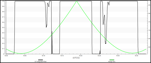
S/T Integrated PDet Range Graph
You are looking for a PDet of 0.8 or greater. It's a given that as distance increases, your PDet will decrease. There are instances where your tracking drops well below a PDet of 0.8. Using the Toggle animation time line button, right-clicking on the graph, and selecting Set Animation Time, you can jump back to the 3D Graphics window to visualize what is occurring.
Overall, the radar system is able to track the aircraft when it's within range and unobstructed by terrain.
Inserting an aerostat into the scenario
You will simulate an aerostat flying near Mount St. Helens. The aerostat is tethered at 10,000 ft above ground level (AGL). An easy way to do this in the STK application, if you're not taking drift into your analysis, is by using a Place (![]() ) object.
) object.
- Bring the Insert STK Objects tool () to the front.
- Insert a Place () object using the Define Properties () method.
- Select the Basic - Position page in the Properties Browser.
- Make the following changes:
- Click .
- Rename the Place3 () Aerostat.
| Option | Value |
|---|---|
| Latitude | 46.1173 deg |
| Longitude | -122.315 deg |
| Height Above Ground | 10000 ft |
Adding a radar jammer to the aerostat
You can model the radar jammer by simply reusing the previously built tracking radar and making a couple of changes.
Copying the Radar object
Copy Servo and paste it on Aerostat so you don't have to model the system from scratch.
- Right-click on Servo () in the Object Browser.
- Select Copy (
 ) in the shortcut menu.
 - Right-click on Aerostat () in the Object Browser.
- Select Paste (
 ).
). - Rename Servo1 () Jam_Servo.
- Rename Tracking_Radar1() Jammer.
Repositioning Jam_Servo
Jam_Servo is attached to Aerostat, but since you copied Servo's properties, it's floating 50 feet above it. Attach Jam_Servo to Aerostat's center point so that it's at the same altitude.
- Open Jam_Servo's () Properties ().
- Select the Basic - Location page.
- Change Location Type to Center.
- Click .
Targeting the airfield search and track radar
When Jammer radiates, you are placing "noise" on Tracking_Radar's receiver.
- Select the Basic - Pointing page.
- Remove (
 ) TestFlight () from the Assigned Targets list.
 - Move () RadarSite () from the Available Targets list to the Assigned Targets list.
- Click .
Viewing your progress in the 3D Graphics window
View the setup in the 3D Graphics window.
- Bring the 3D Graphics window to the front.
- Zoom To Aerostat ().
- Zoom out until you an see both TestFlight and RadarSite.

Aerostat
Defining the radar jammer's antenna
Aerostat is tethered at 10,000 ft AGL. Jam_Servo is attached to Aerostat's center point and is targeting RadarSite. Update Jammer's specifications to differentiate it from the tracking radar.
- Open Jammer's () Properties ().
- Select the Basic - Definition page in the Properties Browser.
- Select the Antenna tab.
- Ensure the Model Specs sub-tab is selected.
- Click the Antenna Model Component Selector ().
- Select Square Horn () in the Antenna Models list when the Select Component dialog box opens.
- Click to close the Select Component dialog box.
- Enter 3 GHz in the Design Frequency field.
- Enter 1 ft in the Diameter field.
Setting the radar jammer's transmitter power
Update the jammer transmitter's power.
- Select the Transmitter tab.
- Ensure the Specs sub-tab is selected.
- Enter 1 W in the Power field.
- Click .
Jamming the radar
The next step is to tell the tracking radar that it's being jammed.
- Open Tracking_Radar's () Properties ().
- Select the Basic - Definition page in the Properties Browser.
- Select the Jamming tab.
- Select the Use check box.
- Select Aerostat/Jam_Servo/Jammer () in the Available Jammer list.
- Move () Aerostat/Jam_Servo/Jammer () to the Assigned Jammers list.
- Click .
Determining the radar jammer's effectiveness
You are now ready to analyze the radar jammer's effectiveness against the tracking radar. Create a custom graph that shows only those contents you are interested in for your analysis. You are interested in S/T Integrated PDet and S/T Integrated PDet w/ Jamming (Search/Track Integrated Probability of detection with jamming).
Creating a new graph
Create a new graph style to plot PDet with jamming.
- Right-click on Tracking_Radar () in the Object Browser.
- Select Access... ().
- Select TestFlight () in the Associated Objects list in the Access Tool.
- Click .
- Select the My Styles () folder in the Styles panel in the Report & Graph Manager.
- Click Create new graph style () in the Styles toolbar.
- Enter PDet Jamming to name your graph.
- Select the Enter key to the set the name and to open the Properties Browser.
Selecting the data providers
Select the data providers and elements for your graph.
- Ensure the Content page is selected in the Properties Browser.
- Expand () the Radar SearchTrack () data provider.
- Insert () the S/T Integrated PDet () data provider element into the Y Axis list.
- Insert () the S/T Integrated PDet w/ Jamming () data provider element into the Y Axis list.
- Click .
Generating the new graph
With your data providers selected, generate your new custom graph.
- Select PDet Jamming () in the My Styles () folder.
- Click .
- Close (
 ) the graph.
By placing the S/T Integrated PDet and S/T Integrated PDet with jamming on the same axis, it's easier to read the graph. As you can see by looking at the graph, the jammer attached to the aerostat is effectively jamming the tracking radar.
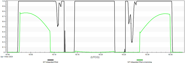
S/T Integrated PDet With Jamming
Generating a radar jamming report
Run a report that will show the radar jammer's affect against the tracking radar. This report will provide a comparison of the probability of detection with or without jamming.
- Return to the Report & Graph manager.
- Select the Radar SearchTrack with Jamming (
 ) report in the Installed Styles () folder.
 - Click .
Four columns of data might be of interest in this report. Start by looking at S/T PDet1 and S/T PDet1 w/Jamming (single pulse) and compare it to S/T Integrated PDet and S/T Integrated PDet w/Jamming. This gives a good example of how integration provides better tracking than single pulse.
Adding a Search/Track Constraint
In the report, you are looking for instances greater than or equal to 0.8 in the S/T Integrated PDet column. Any instance greater than or equal to 0.8 is when the Tracking_Radar can see TestFlight. Add a Min Integrated PDet constraint to Tracking_Radar.
- Open Tracking_Radar's () Properties ().
- Select the Constraints - Active page.
- Click Add new constraints (
 ) in the Active Constraints toolbar.
 - Select Integrated PDet in the Constraint Name list when the Select Constraints to Add dialog box opens.
- Click .
- Click to close the Select Constraints to Add dialog box.
- Enter 0.8 in the Min field in the Integrated PDet panel in the Constraint Properties section
- Click .
Refreshing your report
Refresh your Radar SearchTrack with Jamming report to see the effects of the new minimum integrated PdDet constraint.
- Bring the Radar SearchTrack with Jamming () report to the front.
- Click Refresh (F5) (
 ) the report's toolbar.
 - Notice that access duration has been reduced, and all S/T Integrated PDet values are equal to or greater than 0.8.
The report is only showing those times when Tracking_Radar (![]() ) is able to track TestFlight (
) is able to track TestFlight (![]() ) based on S/T Integrated PDet without jamming. This makes it easier to compare those times against the effects of the jamming radar.
) based on S/T Integrated PDet without jamming. This makes it easier to compare those times against the effects of the jamming radar.
Determining when the radar jammer is effective
You can further modify the report by selecting the Integrated PDet Jamming constraint and enabling the Min field with a value of 0.8. This would show when the radar jammer is effective.
- Return to Tracking_Radar's () Properties ().
- Click Add new constraints () in the Active Constraints toolbar.
- Select Integrated PDet Jamming in the Constraint Name list in the Select Constraints to Add dialog box.
- Click .
- Click to close the Select Constraints to Add dialog box.
- Enter 0.8 in the Min field, located in the Integrated PDet Jamming panel.
- Click .
Refreshing your report
Refresh the report to show those times when the radar jammer is affecting your link.
- Bring the Radar SearchTrack with Jamming report to the front.
- Click Refresh (F5) () the report's toolbar.
Saving your work
Save your work and close out of your scenario.
- Close any open reports, properties and tools.
- Save () your work.
Summary
This scenario determined that a ground-based tracking radar successfully tracked a small aircraft in mountainous terrain. For the most part, tracking was successful except in those instances when the plane was behind the mountains. The second half of the scenario determined that an aerostat radar jamming system effectively jammed the ground-based radar. Based on the radar jammer's specifications, you know that the jammer worked well against the tracking radar.
On your own
Try adjusting the tracking radar's pulse count, frequency or PRF. Different combinations will effect the tracking radar's efficiency. Incrementally increase the jammer transmitter's power by 1 watt at a time to find the power needed to completely jam the tracking radar.