STK Pro, STK Premium (Air), STK Premium (Space), or STK Enterprise
You can obtain the necessary licenses for this tutorial by contacting AGI Support at support@agi.com or 1-800-924-7244.
The results of the tutorial may vary depending on the user settings and data enabled (online operations, terrain server, dynamic Earth data, etc.). It is acceptable to have different results.
Capabilities covered
This lesson covers the following capability of the Ansys Systems Tool Kit® (STK®) digital mission engineering software:
- STK Pro
Problem statement
Engineers and operators need a quick way to determine if structures or vehicles affect visibility between sites, vehicles, or satellites. This gives insight into communications, imaging, radar, and general situational awareness. You are testing a satellite tracking sensor, which is being deployed on board a ship. You need to determine how much of the sensor is blocked by the ship's superstructure and that will affect the sensor's performance.
Solution
Use the AzEl Mask tool to determine the extent to which the ship's superstructure interferes with the sensor's access to the satellite.
What you will learn
Upon completion of this tutorial, you will understand how to:
- Create a body mask file with the AzEl Mask tool
- Use a body mask file for a sensor AzEl Mask constraint
- Visualize the sensor AzEl Mask constraint in the 3D Graphics window
Creating a new scenario
First, you must create a new STK scenario, then build from there.
- Launch the STK application (
 ).
). - Click
 Create a Scenario in the Welcome to STK dialog box.
 - Enter the following in the STK: New Scenario Wizard:
- Click when you finish.
- Click Save (
 ) when the scenario loads.
 - Verify the scenario name and location in the Save As dialog box.
- Click .
| Option | Value |
|---|---|
| Name | AzElMaskTool |
| Location | Default |
| Start | 24 Jul 2024 16:00.00.000 UTCG |
| Stop | + 1 day |
A folder with the same name as your scenario is created for you.
Save () often during this lesson!
Disabling streaming terrain
By default, the STK application connects to the Ansys Geospatial Data Cloud to distribute Earth terrain data for analysis and visualization. Turn off
- Right-click on AzElMaskTool () in the Object Browser.
- Select Properties (
 ) in the shortcut menu.
 - Select the Basic - Terrain page when the Properties Browser opens.
- Clear the Use terrain server for analysis check box in the Terrain Server panel.
- Click to confirm your change and to close the Properties Browser.
Modeling the satellite
For this scenario, you will model a notional satellite in a circular orbit. Circular orbits have a constant radius.
Inserting a Satellite object
A Satellite object models the properties and behavior of a vehicle in orbit around a central body.
- Bring the Insert STK Objects tool (
 ) to the front.
 - Select Satellite (
 ) in the Select An Object To Be Inserted list.
 - Select the Orbit Wizard (
 ) in the Select A Method list.
 - Click .
Using the Orbit Wizard
The Orbit Wizard is a satellite-level tool designed to assist you in creating any one of several standard orbits, or designing your own satellite orbit.
- Enter TestSat in the Satellite Name field when the Orbit Wizard opens.
- Enter 750 km in the Altitude field in the Definition panel.
- Click to propagate the satellite and to close the Orbit Wizard.
Modeling the test ship
The test ship is holding a stationary position in the North Atlantic Ocean.
Inserting a Ship object
A
- Bring the Insert STK Objects tool () to the front.
- Insert a Ship object (
 ) using the Insert Default () method.
 - Right-click on Ship1 () in the Object Browser.
- Select Rename in the shortcut menu.
- Rename Ship1 () TestShip.
Defining the ship's route options
- Open TestShip's () Properties ().
- Select the Basic - Route page when the Properties Browser opens.
- Keep the Propagator set to the default GreatArc method.
- Open the Route Calculation Method drop-down list.
- Select Specify Time.
- Open the Reference drop-down list in the Altitude Reference panel.
- Select WGS84.
The
The Specify Time method allows you to set the Time properties of each waypoint forming the ship's route.
Since you've disabled analytical terrain, you want the ship to sit on the surface of the WGS84 ellipsoid.
Defining the ship's waypoints
The waypoints that comprise the great arc route are contained in a table that displays each point, along with all of its properties, in sequence.
- Click .
- Set the following options for the first waypoint:
Option Value Latitude 31.0 deg Longitude -70.5 deg - Click again.
- Set the second waypoint's Time to 25 Jul 2024 16:00.00.000 UTCG.
- Click to confirm your changes and to close the Properties Browser.
The Latitude and Longitude will be duplicated for the second waypoint.
You want to be sure the ship remains stationary for the duration of your one-day analysis period.
Modeling the ship's satellite tracking sensor
The tracking sensor is mounted in a radome atop the ship's superstructure.
Inserting a Sensor object
A
- Bring the Insert STK Objects tool () to the front.
- Insert a Sensor (
 ) object using the Insert Default () method.
 - Select TestShip () when the Select Object dialog box opens.
- Click to confirm your selection and to close the Select Object dialog box.
- Rename Sensor1 () SatTracker.
Viewing TestShip in the 3D Graphics window
Zoom to TestShip in the 3D Graphics window, which will allow you to view changes to SatTracker.
- Bring the 3D Graphics window to the front.
- Right-click on TestShip () in the Object Browser.
- Select Zoom To in the shortcut menu.
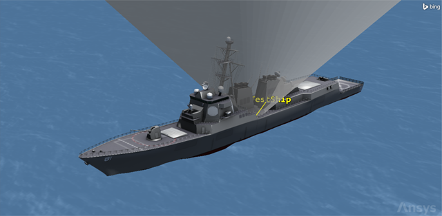
TestShip and attached tracking sensor
By default, SatTracker is attached to TestShip's center point. To model SatTracker correctly using the AzEl Mask tool, you need to move it to the location on TestShip where it is actually located.
Positioning the sensor on the model
The sensor's
- Open SatTracker's () Properties ().
- Select the Basic - Location page when the Properties Browser opens.
- Open the Location Type drop-down list.
- Select Fixed.
- Leave the Type set to Cartesian in the Fixed Location panel.
- Set the following Cartesian coordinates:
- Click to confirm your changes and to keep the Properties Browser open.
- Bring the 3D Graphics window to the front to view the new location of SatTracker ().
With a fixed location type, the location of the sensor is defined using a fixed displacement vector with respect to the parent object's body frame. The displacement can be defined using either Cartesian or Spherical coordinates, which are in the sensor's parent body frame.
| Option | Value |
|---|---|
| X | 25 m |
| Y | -3.5 m |
| Z | 21.3 m |
You could also select 3D Model as the Location Type and use the ship model's attach points or the sensor's
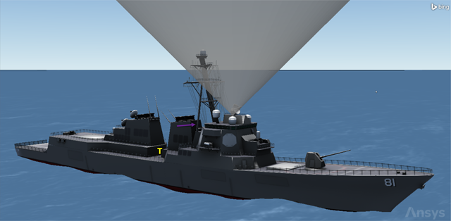
New sensor location
You can see that SatTracker is now located at the correct position on TestShip.
When you position a sensor origin, make certain that it is outside the shell of the 3D model; otherwise the AzEl Mask tool will not work.
Using a Complex Conic sensor type
- Return to SatTracker's () Properties ().
- Select the Basic - Definition page.
- Open the Sensor Type drop-down list.
- Select Complex Conic.
- Enter 180 deg in the Outer field in the Half Angles panel.
- Click to confirm your changes and to close the Properties Browser.
Creating a baseline Access report
Use the
- Right-click on SatTracker () in the Object Browser.
- Select Access... (
 ) in the shortcut menu.
 - Select TestSat () in the Associated Objects list when the Access tool opens.
- Click
 .
. - Click in the Reports panel.
- Note the Total Duration when the Access report opens.
- Keep the Access report open.
- Close the Access tool.
This number is your benchmark.
Creating a body mask with the AzEl Mask tool
There are several ways of applying an azimuth-elevation mask to a sensor. For this tutorial, you will create a body mask. The term body masking refers to the line-of sight-obstruction caused by the three-dimensional model of the parent object of the sensor or other objects in the scenario. A body mask file (*.bmsk) file represents obstructions to visibility from the point of view of the sensor. It is an ASCII text file formatted for compatibility with the STK application that ends in a .bmsk extension. It provides data used to restrict visibility to a sensor. Use the AzEl Mask tool to generate a body mask file. The tool builds the body mask from images of 3D object models and central body shapes as seen from the center of the sensor via perspective projection. It relates the mask by processing images on all six sides of a 3D cube, which overlap slightly to ensure correct processing at the boundaries. The mask consists of one or several contours encoded in AzEl space on each side of the cube, where each contour follows along the boundary of the image of an obstruction. The AzEl mask is built by observing in all directions around the sensor regardless of its field of view. The obscuration contours are constructed using an edge-detection algorithm and stored along with information describing the orientation of the view from which they were constructed. This permits independent setting of visibility limitations in the Access tool calculations using Field of View and Sensor AzEl Mask constraints.
Opening the AzEl Mask tool
You can access the AzEl Mask tool from the Sensor menu in the Menu Bar.
- Select SatTracker () in the Object Browser.
- Select the Sensor menu in the Menu Bar.
- Select AzEl Mask....
Using the AzEl Mask tool
Start by setting up the AzEl Mask tool prior to creating a body mask file. The AzEl Mask tool contains two parts:
- The Az/El Mask View window allows you to see the obscuring objects in the six views used in generating the contours.
- The AzEl Mask dialog box enables you to identify obscuring objects and define the instant in time at which obscuration contours are computed. The time at which obscuration contours are computed is independent of the current animation time and may be important in cases where the parent body has articulating parts or if objects other than the sensor parent body are considered as obstructions.
Select TestShip as the obscuring object and set the Az/El Mask View window's dimensions to 500 pixels per side.
- Move the AzEl Mask for SatTracker dialog box to the right so that it isn't on top of the Az/El Mask View window, if needed.
- Select TestShip () in the Obscuring Objects list.
- Enter 500 in the Window Dim field in the Data panel.
- Leave the Do not render normal 3D windows while computing check box selected in the Rendering panel.
- Click to confirm your changes and to keep the AzEl Mask tool open.
This is the height and width, in pixels, of the window used to generate the body mask. Larger window sizes produce more accurate masks, which require more access computation time.
A mask file cannot be generated if the window dimensions are too small or if they are larger than the STK workspace. If a Window Dim value of 500 places this window outside of your STK workspace — for example, if you have a small screen size — decrease the value until it fits inside the STK workspace.
This will stop the rendering in the 3D Graphics window when the tool is computing data, which can improve the speed of the computations.
Creating a body mask file
You can now create a static body mask file to use for visualization and analysis.
- Click .
- Ensure your body mask file will be saved in your scenario folder (for example, C:\Users\<username>\Documents\STK_ODTK 13\AzElMaskTool) when the Select Body Mask File dialog box opens.
- Use the default File name (SatTracker.bmsk).
- Click .
- Close (
 ) the Az/El Mask View window when the computations are complete to close both it and the AzEl Mask dialog box.
The six views used to construct the mask will be shown in successive fashion when you save your body mask file. You can see outlines of the ship's mast and radar dish.
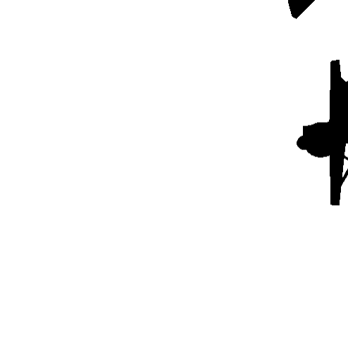
AzEl Mask View Window
Viewing the body mask file
Take a look at the contents of your body mask file to better understand what it will do. The file contains data groups and data elements to ensure that the data contained in the file can be read by the STK application. A data group identifies a group of related quantities that are specified on the same time grid. The information contained in each data group consists of keywords their associated values, which are called keyword phrases. Individual values are specified using data elements.
- Open Windows File Explorer.
- Navigate to your scenario folder (for example, C:\Users\<username>\Documents\STK_ODTK 13\AzElMaskTool).
- Open SatTracker.bmsk with the text editor of your choice (for example, Windows Notepad or Notepad++).
- Scroll through the file contents.
- Note the MaxAngleBetweenSamples data element is specified as 5.0000000000000000e+00, the default value.
- Note the Exclusion and Inclusion data groups.
- Note the comments in each of these data groups indicating along which direction the inclusion and exclusion zones are generated and the LocalZ and LocalX keyword phrases.
- Note the NumAzElPairs keyword phrases and the AzElPairs data groups.
- Close your text editor without making any changes when you are finished.
- Return to the STK application.
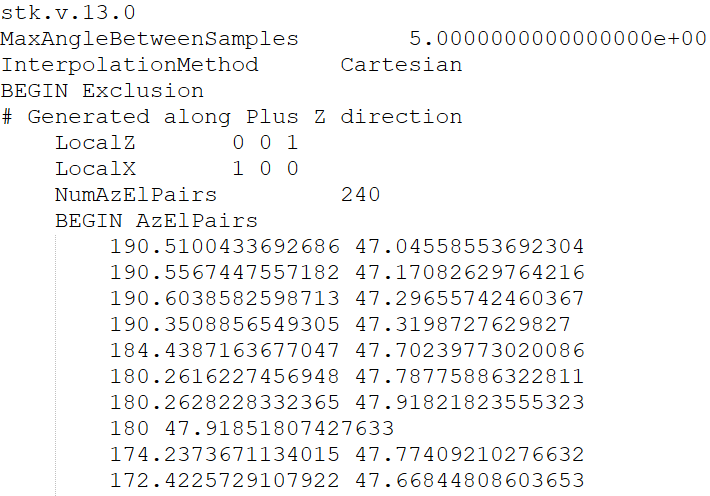
Body Mask File Contents
Additional points on the obstruction boundary, as determined using the interpolation method, were added whenever the angular separation between points in the file was greater than this setting. The additional points provide better accuracy in access computations using the body mask constraint.
Whereas an
The latter keyword phrases specify the relationship between the Z and X axes used in the description of the Az/El coordinates and the body frame of the parent object of the sensor. Elevation is measured as the angle out of the local X-Y plane, positive in the direction of +Z. Azimuth is measured as the angle in the local X-Y plane from X positive in the direction of Y.
Points along an exclusion or inclusion boundary are identified by groups of azimuth/elevation coordinate pairs, where the angles are measured in a local reference frame that is related to the mask references axes frame by the local axis directions specified with the contour. The NumAzElPairs data element specifies the maximum number of azimuth/elevation coordinate sets to follow in the respective AzElPairs data group.
Applying the body mask file to SatTracker
You can apply the body mask file to SatTracker as an access constraint by updating the
Constraining SatTracker with the body mask file
Apply the body mask file as an access constraint.
- Open SatTracker's () Properties ().
- Select the Basic - Sensor AzEl Mask page when the properties browser opens.
- Open the Use drop-down list.
- Select MaskFile.
- Click the Mask File ellipsis (
 ).
). - Browse to your scenario folder (for example, C:\Users\<username>\Documents\STK_ODTK 13\AzElMaskTool) when the Select File dialog box opens.
- Select SatTracker.bmsk.
- Click to confirm your selection and to close the Select File dialog box.
- Select the Use Mask for Access Constraint check box.
- Click to confirm your changes and to keep the Properties Browser open.
This will enable the Sensor Az-El Mask constraint, which you can confirm is selected on the
Visualizing SatTracker's AzEl Mask constraint
In order to visualize the constraint that SatTracker is using, you have to define which constraint is used to modify its field of view. Use SatTracker's 2D Graphics Projection Graphics properties to control the display of its projection graphics in the 2D and 3D Graphics windows.
- Select the 2D Graphics - Projection page.
- Select the Use Constraints check box in the Field of View panel.
- Select SensorAzElMask in the list.
- Click to confirm your changes and to keep the Properties Browser open.
Defining the 3D Graphics Projection properties
SatTracker's 3D Graphics Projection properties are used to control the display of its cone into space as well as the its extension into space. This is a visualization property, not an analytical property.
- Select the 3D Graphics - Projection page.
- Enter 30 m in the Space Projection field in the Extension Distances panel.
- Click to confirm your changes and to close the Properties Browser.
Extension distances define the length of SatTracker's projection. In this case, the distance is computed so that the projection of the outermost point on the contour along the bore sight is equal to the distance entered.
Visualizing the body mask in the 3D Graphics window
You can now view the body mask in the 3D Graphics window.
- Bring the 3D Graphics window to the front.
- Maximize your 3D Graphics window.
- Zoom to TestShip ().
- Use your mouse to zoom out until you can the whole ship and some of the body mask.
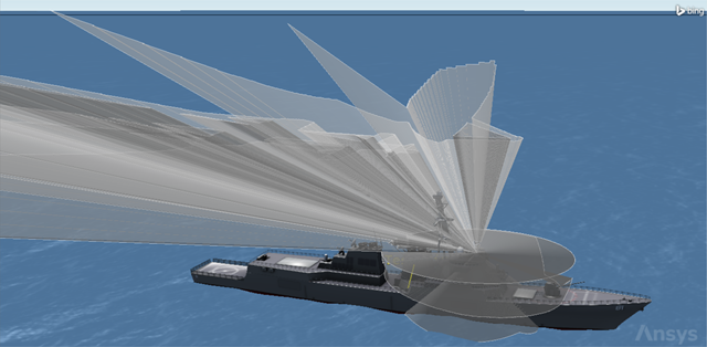
TestShip body mask
You can see that SatTracker's field of view is being blocked by elements of TestShip's superstructure.
Refreshing the Access report
Refresh your Access report to take into account the constraints imposed by the body mask file.
- Bring your Access report to the front.
- Click Refresh (F5) (
 ) on the report toolbar.
 - Note the Total Duration.
Without taking the ship's superstructure into account, the original total access was nearly a quarter of an hour longer. It is evident the superstructure reduces the amount of time that you can track the satellite by a significant extent.
- Close the Access report when finished.
Saving your work
Clean up your workspace and close out your scenario.
- Close any open reports, properties and tools.
- Save () your work.
Summary
You modeled a ship deploying a sensor that tracks satellites. You propagated a single, notional satellite, then you used a Sensor object to model the field of view of the sensor and attached it to a 3D model of the ship. You then generated an Access report between the sensor and the satellite to create a benchmark access duration. You then used the AzEl Mask tool to create a body mask file to account for ship's superstructure, which obscured portions of the sensor's field of view. Finally, you refreshed your access report, which allowed you to determine the extent to which the ship's superstructure affected your overall access duration.