Part 18:
STK Premium (Space) or STK Enterprise
You can obtain the necessary licenses for this tutorial by contacting AGI Support at support@agi.com or 1-800-924-7244.
Required Capability Install: For versions 12.10 and earlier of the STK software, this lesson requires the installation of the EOIR capability. For these versions of the software, the EOIR installer is included in the STK Premium software download, but requires a separate installation process. Read the Readme.htm found in the STK software install folder for installation instructions. You can obtain the necessary install by visiting https://support.agi.com/downloads or calling AGI support.
This tutorial requires version 12.9 of the STK software or newer to complete in its entirety. If you have an earlier version of the STK software, you can view a legacy version of this lesson.
The results of the tutorial may vary depending on the user settings and data enabled (online operations, terrain server, dynamic Earth data, etc.). It is acceptable to have different results.
Capabilities covered
This lesson covers the following capabilities of the Ansys Systems Tool Kit® (STK®) digital mission engineering software:
- STK Pro
- Electro-Optical Infrared Sensor Performance (EOIR)
- STK SatPro
Problem statement
Engineers and operators require a fast and easy way to model and simulate detection, tracking, and imaging performance of electro-optical and infrared sensors. You want to simulate tracking a polar satellite that is in a low Earth orbit (LEO) from an observatory located in Hawaii. You want to model the facility's telescope from specifications and take atmospheric effects, temperature, emissivity, and radiance into consideration for your analysis.
Solution
Use the STK application and the Electro-Optical Infrared Sensor Performance (EOIR) capability to model, simulate, and analyze a synthetic sensor scene from the 1.6-meter Advanced Electro-Optical System (AEOS) telescope at the Air Force Maui Optical Station (AMOS) observatory located at the Maui Space Surveillance Complex (MSSC) in Maui, Hawaii, that is tracking a polar satellite in LEO.
What you will learn
Upon completion of this tutorial, you will understand:
- How to configure Sensor objects to use the EOIR sensor type
- How to create an EOIR sensor scene
- How to view data in the EOIR Scene Visual Details dialog box
- How to create a custom EOIR signal-to-noise (SNR) graph
Creating a new scenario
First, you must create a new STK scenario, and then build from there.
- Launch the STK application (
 ).
). - Click
 Create a Scenario in the Welcome to STK dialog box.
 - Enter the following in the STK: New Scenario Wizard:
- Click when you finish.
- Click Save (
 ) when the scenario loads. The STK application creates a folder with the same name as your scenario for you.
 - Verify the scenario name and location in the Save As window.
- Click .
| Option | Value |
|---|---|
| Name | STK_EOIR |
| Location | Default |
| Start | 1 Aug 2024 15:00:00.000 UTCG |
| Stop | + 10 min |
Save (![]() ) often during this lesson!
) often during this lesson!
Modeling the AEOS telescope
Add the AEOS 1.6-meter diameter telescope to your scenario.
Inserting a Facility object
Use the Insert STK Objects tool to
- Bring the Insert STK Objects tool (
 ) to the front.
 - Select Facility (
 ) in the Select An Object To Be Inserted list.
 - Select the From Standard Object Database (
 ) method.
 - Click .
Selecting the MSSC 1.6-meter telescope for the Facility object
Search for select the MSSC 1.6-meter telescope to use for the Facility object.
- If you have online operations enabled, clear the Online check box in the Data Sources.
- This will ensure you only select the MSSC facility available in your local object database.
- Click .
- Select MSSC 1.6m in the Results list that uses the Local Database Data Source.
- Click .
- Click to close the Search Standard Object Data dialog box.
Enter MSSC in the Name field in the Search Standard Object Data dialog box.
Inserting a Sensor object
Add a sensor to MSSC_1_6m Facility object to model the 1.6-meter AEOS telescope.
- Insert a Sensor (
 ) object using the Insert Default () method.
 - Select MSSC_1_6m () in the Select Object dialog box.
- Click .
- Right-click on Sensor1 () in the Object Browser.
- Select Rename in the shortcut menu.
- Rename Sensor1 () Telescope.
Creating an EOIR sensor
The
Selecting the EOIR sensor type
Start by selecting the EOIR sensor type on the sensor's
- Right-click on Telescope () in the Object Browser.
- Select Properties (
 ) in the shortcut menu.
 - Select the Basic - Definition page when the Properties Browser opens.
- Select EOIR in the Sensor Type drop-down list.
- Click to accept your change and to keep the Properties Browser open.
Setting the sensor's spatial properties
When you choose EOIR as the sensor yype, you can select the Spatial tab to specify its spatial properties. The default input setting is Field-of-View and Number of Pixels. Update these spatial properties to define the total field-of-view angles to more accurately model the AEOS telescope.
- Ensure the Spatial tab is selected on the Basic - Definition page.
- Set the following parameters in the Field of View panel:
- Review the settings in the Number of Pixels panel.
- Click .
| Option | Value |
|---|---|
| Horizontal Half Angle | 7.5 deg |
| Vertical Half Angle | 7.5 deg |
The EOIR capability uses these half angles to determine the full angular extent of the sensor field of view (FOV).
These are the number of sensor pixels in the field of view in the horizontal and vertical directions. The default value is 128 for each direction.
The Related Detector Parameters and Instantaneous Field of View values are based on the sensor spatial and optical properties. These are read-only fields and are automatically updated when you apply your changes.
Setting the sensor's spectral properties
The AEOS telescope observes the long infrared waveband. Specify the sensor's
- Select the Spectral tab on the Basic - Definition page.
- Set the following parameters (in micrometers) in the Spectral Band Edge Wavelengths panel:
- Leave the Number Of Intervals set at 6.000000.
- Leave the Spectral Shape set to the Use Optical and Radiometric Response option.
- Click .
You must set the High value first.
| Option | Value |
|---|---|
| High | 1.0 |
| Low | 0.7 |
This defaults the spectral shape to the individual optical transmission and quantum efficiency spectral characteristics.
Setting the sensor's optical properties
Next, set the sensor's optical properties. You will specify the F Number (Effective Focal Length / Effective Pupil Diameter) and the diameter (in cm) of the "single lens equivalent" optical prescription.
- Select the Optical tab on the Basic - Definition page.
- Select F-Number and Entrance Pupil Diameter for the Input.
- Set the following parameters:
- Select Negligible Aberrations in the Image Quality drop-down list.
- Click .
| Option | Value |
|---|---|
| F/# | 200 |
| Entrance Pupil Diameter | 367.00 |
The EOIR capability models aberrations based on a root-mean-square wavefront error. The Negligible Aberrations setting introduces a 7% wave front error.
Setting the sensor's radiometric properties
You can populate and edit sensor performance data with measurements from an actual sensor. The sensor's radiometric properties define the noise floor and the saturation ceiling. When preparing to take measurements with the sensor model, you specify an integration time. This is the time interval over which a radiant signal is collected before generating an image. The longer the time, the more photons that get collected. This field is equivalent to the "exposure time" setting on an analog film camera.
You can also define a set of points that relate Integration (Exposure) Time to NEI/SEI (noise equivalent irradiance / saturation equivalent irradiance). The STK software linearly interpolates between the points to get correct NEI/SEI for the integration time you set.
- Select the Radiometric tab on the Basic - Definition page.
- Set the following options in the Sensitivity panel:
- Notice that Processing Level defaults to Sensor Output.
- Enter 1 in the Line of Sight Jitter field in the Jitter panel.
- Click to apply your changes and to close the Properties Browser
| Option | Value |
|---|---|
| Integration Time | 100 |
| Equivalent Value | 1e-16 |
The Sensitivity defines the "noise floor" of the sensor. The sensor will not detect signals below this level.
Processing levels enable you to visualize the geometric information in the sensor scene or the sensor output image. The Radiometric Input simulates the light entering the sensor lens before hitting the sensor detector when generating the EOIR sensor scene.
This introduces a Gaussian vibration of one milliradian along the sensor boresight.
Opening the EOIR toolbar
Before you can use the EOIR capability with your sensor, you must first display the EOIR toolbar. You can use the
- Select View in the Menu Bar.
- Select Toolbars in the View menu.
- Select EOIR in the Toolbar submenu to show the EOIR toolbar.

Eoir toolbar
Viewing the EOIR Configuration
View the sensor's
- Click EOIR Configuration... (
 ) in the EOIR toolbar.
 - Click to close the EOIR Configuration dialog box.
This displays the sensor's EOIR Configuration dialog box. All central bodies and objects, except for the source sensor, that are part of the EOIR Configuration are listed in the available target list.
Generating an EOIR sensor scene
Now you are ready to
- Select Telescope () in the Object Browser.
- Click EOIR Sensor Scene... (
 ) in the EOIR toolbar.
 - Right-click on the sensor scene.
- Select Details... in the shortcut menu.
- Move the EOIR Scene Visual Details dialog box so that it's not sitting on top of the sensor scene.
- Select the BGRY option in the Color Map panel.
- Click .
- Click around the scene to display information on the EOIR Scene Visual Details window for each pixel.
- Click one of the stars to get more details on this object.
- Close the EOIR Scene Visual Details dialog box and the EOIR Sensor Scene window when finished.
This generates an image that represents the radiometric input to the sensor. You will see some white dots and gray dots against a black background.
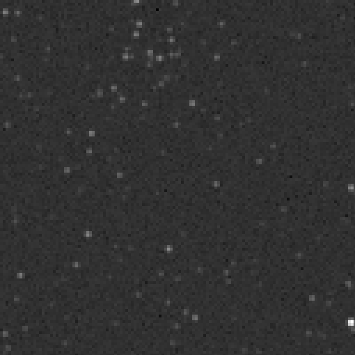
EOIR Sensor SCENE in GrayScale
The input scene represents the analog world by digitally sampling the "modeled universe" at 4 times the sensor's pixel's spatial frequency, 16 spatial samples per sensor pixel, and over the passband and at wavelengths defined by the sensor model. The input scene is thus a "box" of floating point numbers of dimension (Horizontal spatial resolution × Vertical spatial resolution × Spectral resolution). These scenes accurately portray sensor images for the processing level selected.
You can use the
EOIR uses false color to bring out details in the image data that are often lost when displayed on a monitor with less resolution than the EOIR sensor. For instance, a typical monitor can display only 256 levels of grayscale, whereas an EOIR sensor might have 4096 levels of grayscale resolution. Color mapping is only for visual effect and does not change any of the internal data values.
For the Sensor Output processing level, the raw sensor data and image can be saved out at every animation step. You can save the data in each sensor click to a file by selecting Pixel Spectral Data on the EOIR Scene Visual Details page. You can then compound these images to create a movie or run through external image processing software for further analysis.

EOIR Sensor SCENE with BGRY color map
Inserting a Satellite object
Insert a Satellite object using the Orbit Wizard to model the polar satellite in LEO that you are tracking.
- Bring the Insert STK Objects tool () to the front.
- Insert a Satellite (
 ) object using the Orbit Wizard (
 ) method.
 - Set the following options in the Orbit Wizard:
- Click to accept your changes and to close the Orbit Wizard.
| Option | Value |
|---|---|
| Type | Circular |
| Satellite Name | LEO_Sat |
| Inclination | 98 deg |
| Altitude | 700 km |
| RAAN | 24 deg |
The orbit will take the satellite through the telescope's field of view.
Viewing LEO_Sat and the ground site in the 3D Graphics window
View the LEO satellite and the Facility in the 3D Graphics window.
- Bring the 3D Graphics window to the front.
- Right-click on LEO_Sat () in the Object Browser.
- Select Zoom To.
- Pan and zoom around so that you can view both LEO_Sat () and MSSC_1_6m ().
- Click Decrease Time Step (
 ) in the Animation toolbar until the Time Step is set to 1 sec.
 - Click Start (
 ) to animate the scenario.
 - Click Reset (
 ) when finished.
Although this tutorial is a ground-to-space example, it is possible to host an EOIR sensor on both air and space vehicles. The work flow of setting up an EOIR sensor model is similar for all supported STK objects.
Viewing LEO_Sat in the EOIR sensor scene
An EOIR sensor will take images of objects that fall within the sensor's field of view that hey are sufficiently bright, either in reflected light or from self-radiance, at wavelengths that the sensor can detect. When LEO_Sat passes over the AMOS facility, AMOS is in darkness while the satellite is illuminated. This scenario gives good lighting conditions for imaging.
Viewing LEO_Sat's basic EOIR shape
With the EOIR capability, you can set image generation properties for selected STK objects. When you open an properties, you will see
- Open LEO_Sat's () Properties ().
- Select the Basic - EOIR Shape page when the Properties Browser opens.
- Examine the following options:
- Shape
- Radius
- Body Temperature
- Temperature
- Material
- Keep the default settings.
- Click to close the Properties Browser.
Adding LEO_Sat to the EOIR configuration
To see the LEO_Sat in the EOIR sensor scene, you must first add it as a target in the EOIR configuration.
- Click EOIR Configuration... () in the EOIR toolbar to open the EOIR Configuration dialog box.
- Double-click on Satellite/LEO_Sat () in the Available STK Objects list to move it to the Selected Targets list.
- Click to close the EOIR Configuration dialog box.
Creating an Access between Telescope and LEO_Sat
Create an access report between Telescope and LEO_Sat. You will use the Access for further analysis.
- Right-click on Telescope () in the Object Browser.
- Select Access... (
 ).
). - Select LEO_Sat () in the Associated Objects list.
- Click
 .
.
Setting animation time from an Access report
Generate an Access report. You will use the time of the first access to set a viewing time for your sensor scene.
- Click in the Reports panel.
- Right-click on the first access start time in the Access report.
- Select Start Time in the shortcut menu.
- Select Set Animation Time in the Start Time submenu.
- Close (
 ) the access report.
 - Close () the Access tool.
This sets the Current Scenario Time in the Animation toolbar to the time when LEO_Sat first enters the telescope's field of view.
Creating the EOIR Sensor Scene
Generate the EOIR scenario scene.
- Select Telescope () in the Object Browser.
- Click EOIR Sensor Scene... () in the EOIR toolbar.
- Right-click on the sensor scene.
- Select Details... in the shortcut menu to open the EOIR Scene Visual Details dialog box.
- Select the Gray Scale option in the Color Map panel.
- Click .
Note that the AGC check box is selected. AGC is Automatic Gain Control. When this option is selected, the EOIR capability automatically calculates brightness and contrast such that the brightest scene detail fits within the brightness resolution of the monitor.
Performing EOIR sensor scene analysis
View the EOIR sensor scene details.
- Decrease () the animation Time Step to 0.5 seconds.
- Step Forward (
 ) the scenario until you see the satellite come into the scene.
 - Click one of the stars and the target satellite to get more details on those objects.
- Click to close the EOIR Scene Visual Details dialog box when finished.
- Close () the EOIR sensor scene.
The dot that represents the satellite moves across the scene while the stars stay relatively still.
Creating custom graphs for EOIR sensors
The EOIR capability does more than simulate scenes created by an EOIR sensor. It can also calculate metrics a sensor would receive from a target's signal. The following will familiarize you with some of the available EOIR data providers.
Creating a new graph
First, create a new graph called Target Metrics.
- Right-click on Telescope () in the Object Browser.
- Select Report & Graph Manager... in the shortcut menu (
 ) to open the Report & Graph Manager.
 - Select the My Styles (
 ) folder in the Styles panel.
 - Click Create new graph style (
 ) in the Styles toolbar.
 - Enter Sensor to Target Metrics.
- Select the Enter key to rename the graph and to open the graph's properties.
Setting the graph's data providers
You will use the
- EOIR Sensor To Target Metrics: time dependent metrics for a unique EOIR Sensor-Band / Target pairing.
- In-band target irradiance: the irradiance at the sensor aperture from a target object whose angular extent is smaller than the effective instantaneous field of view, i.e. a point source target
- Signal to noise ratio: is the ratio of the difference in sensor response between target-containing pixel(s) and the local surrounding pixels to the total noise. For point source targets the background is assumed to be uniform (spatial clutter is neglected) and the target is assumed to be exactly centered on a pixel.
- Expand (
 ) the EOIR Sensor To Target Metrics () data provider in the Data Provider list.
 - Move (
 ) the In-band target irradiance (
 ) data provider element to the Y Axis list.
 - Move () the Signal to noise ratio () data provider element to the Y2 Axis list.
- Select EOIR Sensor to Target Metrics-In-band target irradiance in the Y Axis list
- Click below the Y2 Axis box to open the Units dialog box.
- Clear the Use Defaults check box.
- Select Power in the Dimension column.
- Select Watts (W) in the New Unit Value list.
- Click to close the Units dialog box.
Setting the step size
Set the graph's step size to one second.
- Enter 1.0 sec in the Step Size field.
- Click to accept your changes and to close the Properties Browser.
Setting the Time properties
Set the time properties so the data is reported over the first Access interval.
- Return to the Report & Graph Manager.
- Select Specify Time Properties in the Time Properties panel.
- Open (
 ) the Start and Stop times drop-down menu.
 - Select Interval Component... to open the Select Time Interval dialog box.
- Select Facility-MSSC_1_6m-Sensor-Telescope-To-Satellite-LEO_Sat (
 ) in the Objects list.
 - Expand () AccessIntervals (
 ) in the Intervals for list.
 - Select First (
 ).
). - Click to close the Select Time Interval dialog box.
This limits the analysis period to the interval when LEO_Sat is visible in the EOIR sensor scene and decreases the computation time needed for the analysis.
Generating the custom graph
Now, generate the custom graph over the first Access interval.
- Select the Sensor to Target Metrics (
 ) in the Styles list.
 - Click .
- Look at the graph.
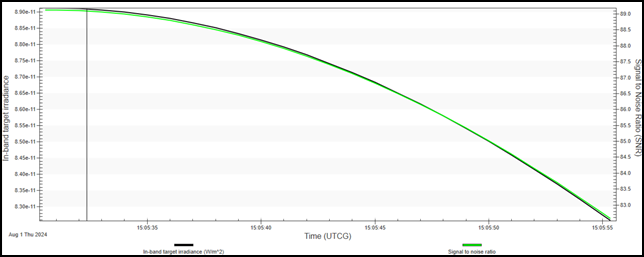
In-band target irradiance versus SNR graph
This graph shows the signal is small relative to the noise, however using gray scale color mapping, you are able to see the target in the scene. Keep the graph open.
Viewing the effects of EOIR atmosphere modeling
By default, the EOIR capability neither applies an atmosphere model nor an atmosphere parameter setting when generating a sensor scene. You will apply a Simple Atmosphere model and adjust its parameters to view the effects the atmosphere has on your data.
Selecting the Simple Atmosphere model
Set the EOIR atmosphere model.
- Click EOIR Configuration... () in the EOIR toolbar to open the EOIR Configuration dialog box.
- Click to open the EOIR Atmosphere, Clouds, and Texture Maps dialog box.
- Take a minute to view the different atmosphere models:
- Simple Atmosphere: This model calculates the atmospheric properties at the wavelengths corresponding to the Spectral Band Edges, and at a spectral resolution specified by the Number of Intervals set on the Sensor's Spectral Properties page. The Simple Atmosphere model only uses variations of atmospheric properties with altitude. It does not calculate the horizontal variations — which constitute weather — nor clouds.
- MODTRAN Derived Lookup Table: MODTRAN is a community standard, and the MODTRAN Derived Lookup Table atmosphere model is one of the highest-fidelity atmospheric models available in EOIR.
- Select the Simple Atmosphere option in the Modes panel.
- Set the following parameters in the Parameters panel:
- Aerosol Models: This selects the type of aerosol model for the Simple Atmosphere model to use. Aerosols are tiny particles in the air that cause whitish haze visible to the human eye. Each aerosol model comprises a distribution of particles of different sizes and how light interacts with them. For instance, in a Maritime atmosphere, salt crystals from wind and wave action are a major contributor to aerosols.
- Visibility: This specifies the meteorological visibility in kilometers. Meteorological visibility is the greatest distance at which a black object of suitable dimensions, located near the ground, can be seen and recognized when observed against a bright background.
- Humidity: This specifies the relative humidity as a percentage from 0.0 to 100.0.
- Click to close the EOIR Atmosphere, Clouds, and Texture Maps dialog box.
- Click to close the EOIR Configuration dialog box.
| Option | Value |
|---|---|
| Aerosol Models | Maritime |
| Visibility | 40 |
| Humidity | 70 |
The Atmosphere Parameters provide some control over the atmosphere's physical characteristics. These characteristics include:
Refreshing the custom graph
Refresh the open graph to see the changes.
- Return to the custom graph.
- Click Refresh (F5) (
 ) in the graph toolbar.
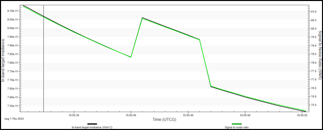
graph showing effects of atmospheric degredaton
The degradation is due to atmospheric effects. Keep the graph open.
Turning off the atmosphere model
Now that you have seen the effects the atmosphere has on your data, turn the atmosphere off.
- Click EOIR Configuration... () in the EOIR toolbar to open the EOIR Configuration dialog box.
- Click to open the EOIR Atmosphere, Clouds, and Texture Maps dialog box.
- Select the Atmosphere Off option in the Modes panel.
- Click to close the EOIR Atmosphere, Clouds, and Texture Maps dialog box.
- Click to close the EOIR Configuration dialog box.
Viewing the effects of a custom EOIR shape
Earlier, you viewed LEO_Sat's basic EOIR Shape properties. Now, update some of those properties to more closely model LEO communications satellite.
Redefining LEO_Sat's EOIR shape
Define the material and shape properties of the satellite.
- Open the LEO_Sat's () Properties ().
- Select the Basic - EOIR Shape page.
- Set the following options:
- LEOComm: the shape is based on the 3D model iridium.glb
- Static: the STK software applies this temperature to the entire shape. This then applies for the entire EOIR scene time period
- Aluminum MLI: multi-layer insulation. Each surface material has optical properties used in the sensor scene calculation. One of these is reflectance. Light bouncing off a surface is selectively reflected by wavelength; i.e., some wavelengths are absorbed instead of reflected. In the visible wavelengths, this is what gives objects color. Each surface naterial has a table of its reflectance versus wavelength.
- Click .
| Option | Value |
|---|---|
| Shape | LEOComm |
| Body Temperature | Static |
| Temperature | 400 K |
| Material | Aluminum MLI |
Regenerating the EOIR sensor scene
Regenerate the EOIR sensor scene with LEO_Sat's updated EOIR Shape properties.
- Right-click at the beginning of the custom graph.
- Select Set Animation Time.
- Select Telescope () in the Object Browser.
- Click EOIR Sensor Scene... () in the EOIR toolbar.
- Right-click on the sensor scene.
- Select Details... in the shortcut menu to open the EOIR Scene Visual Details dialog box.
Viewing LEO_Sat in the EOIR sensor scene
You can view how LEO_Sat now appears in the EOIR Sensor Scene window.
- Step Forward () to see the satellite move across the scene.
- Click on the target satellite to view information about it.
- Click to close the EOIR Scene Visual Details dialog box when finished.
Note that LEO_Sat's updated EOIR Shape properties, including the Temperature and Material, now display in the Scene Pick Information panel.
Refreshing the custom graph
Refresh the custom graph to see how the updated properties affect it.
- Return to the custom graph.
- Click Refresh (F5) () in the graph toolbar.
graph showing effects of EOIR shape changes
The curve is showing a single minimum rate in in-band target irradiance and SNR that coincides with the satellite passing near the facility's zenith.
Analyzing the light signature of a tumbling satellite
In your previous analysis, the satellite was holding a nadir-pointing
Updating the satellite's Attitude properties
Update LEO_Sat's attitude profile to be that of a
- Open the LEO_Sat's () Properties ().
- Select the Basic - Attitude page.
- Set the following options:
- Click to accept your changes and to close the Properties Browser.
| Option | Value |
|---|---|
| Type | Precessing Spin |
| Body Spin Axis | Type: Cartesian X: 0 Y: 1 Z: 0 |
| Precession - Rate | 30 revs/min |
| Spin - Rate | 30 revs/min |
Viewing LEO_Sat in the 3D Graphics window
View LEO_Sat spinning in the 3D Graphics window.
- Bring the 3D Graphics window to the front.
- Zoom To LEO_Sat ().
- Decrease () the animation Time Step to 0.1 seconds.
- Step Forward () to see the satellite tumble.
Updating the custom graph
Refresh your custom graph and update its step size to better show the tumbling satellite.
- Return to your custom graph.
- Click Refresh (F5) () in the graph toolbar.
- Enter 0.1 sec in the Step field.
- Select the Enter key.
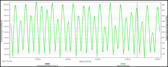
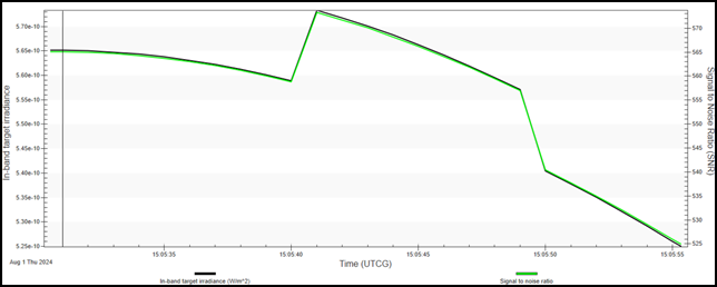
graph showing tumbling satellite
As the spacecraft rotates, various panels reflect varying amounts of light. The pot is jagged, thus confirming that the spacecraft is tumbling.
Saving your work
Clean up your workspace and save your scenario.
- Close any open reports, properties and tools which are still open.
- Save () your work.
Summary
This was an introduction to the STK software's EOIR capability. You modeled, simulated, and analyzed the MSSC's 1.6-meter AEOS telescope at the AMOS observatory in Maui, Hawaii, that tracked a polar satellite in LEO. You set your Sensor object attached to the ground site to use the EOIR capability. You set its spatial, spectral, optical, and radiometric properties. Using the EOIR sensor scene, you obtained data on stars and the LEO satellite. You became familiar with satellite EOIR shape configurations and attitude issues. Using the EOIR configuration, you applied atmospheric changes to your analysis. You created a custom graph and graphed the various changes to your analysis.