STK Premium (Air) or STK Enterprise
You can obtain the necessary licenses for this tutorial by contacting AGI Support at support@agi.com or 1-800-924-7244.
Required Software Install: This lesson uses the MATLAB programming platform for analysis. You must install MATLAB in order to complete this tutorial.
Required Auxiliary Extension Install: This lesson requires the installation of a
This tutorial requires version 12.10 of the STK software or newer to complete in its entirety.
The results of the tutorial may vary depending on the user settings and data enabled (online operations, terrain server, dynamic Earth data, etc.). It is acceptable to have different results.
Capabilities and tools covered
This lesson covers the following capabilities and tools of the Ansys Systems Tool Kit® (STK®) digital mission engineering software:
- STK Pro
- Aviator
- Aviator Pro
- Radar
- Integration
- Air Rendezvous Simulation Tool
Problem statement
Engineers and technicians require a quick and easy way to simulate the flight profiles of one aircraft flying in the lead position and another aircraft, which rendezvous with the lead aircraft, flying in a chase position. They want to model a variety of aerial maneuvers as part of a simulated radar run. The lead aircraft is modeled with a notional radar cross section, while the chase aircraft is equipped with a model radar system that tracks off its nose from ±60 degrees azimuth and from ±45 degrees elevation. A way to simulate radar runs will be essential to the design of the radar system and analyzing the radar cross section of the lead aircraft.
Solution
Use the STK application's core capabilities and the Aviator Pro capability's Air Rendezvous Simulation Tool to create specialized stopping conditions to feed Aviator maneuvers to both of your aircraft. With this tool, you can collect radar statistics by following the lead aircraft from a range of azimuth, elevation, and range values.
What you will learn
Upon completion of this tutorial, you will understand the following:
- How to use the Air Rendezvous Simulation Tool
- How to interpret radar statistics
Using a starter scenario
To speed things up and allow you to focus on the portion of this exercise that teaches you how to use the Air Rendezvous Simulation tool, a partially created scenario has been provided for you. Depending on your version of the STK software, you can access it in one of two ways.
Opening the starter scenario in version 13 of the STK software or newer
If you are using version 13 of the STK software or newer, the starter scenario is included in your install.
- Launch the STK application (
 ).
). - Click
 Open a Scenario in the Welcome to STK dialog box.
 - Browse to <Install Dir>\Data\Resources\stktraining\VDFs.
- Select AirRendezvousSimulationTool.vdf.
- Click .
Downloading the starter scenario for version 12.10 of the STK software
If you are using version 12.10 of the STK software, you must download the starter scenario from AGI.com.
- Download the zipped folder here: https://support.agi.com/download/?type=training&dir=sdf/help&file=AirRendezvousSimulationTool.zip
- Navigate to the downloaded folder.
- Right-click on AirRendezvousSimulationTool.zip.
- Select Extract All... in the shortcut menu.
- Set the Files will be extracted to this folder: path to the location of your choice. The default path is C:\Users\<username>\Downloads\AirRendezvousSimulationTool.
- Click .
- Go to the chosen folder.
- Double-click on AirRendezvousSimulationTool.vdf to open the starter scenario in the STK application.
If you are not already logged in, you will be prompted to log in to agi.com to download the file. If you do not have an agi.com account, you will need to create one. The user approval process can take up to three (3) business days. Please contact support@agi.com if you need access sooner.
AirRendezvousSimulationTool.vdf will be in the extracted folder.
Saving the VDF as a scenario
Save and extract the VDF data in the form of a scenario folder. When you save a VDF in the STK application, it will save in its originating format. That is, if you open a VDF, the default save format will be a VDF (.vdf). If you want to save and extract a VDF as a scenario folder, you must change the file format by using the Save As feature. This will create a permanent scenario file complete with child objects and any additional files packaged with the VDF.
- Open the File menu when the starter scenario opens.
- Select Save As....
- Select the STK User folder in the navigation pane when the Save As dialog box opens.
- Select the AirRendezvousSimulationTool folder.
- Click .
- Select Scenario Files (*.sc) in the Save as type drop-down list.
- Select the AirRendezvousSimulationTool Scenario file in the file browser.
- Click .
- Click in the Confirm Save As Dialog box to overwrite the existing scenario file in the folder and to save your scenario.
A scenario folder with the same name as the VDF was created for you when you opened the VDF in the STK application. This folder contains the temporarily unpacked files from the VDF.
When saving a VDF as a scenario folder, you should extract its contents to the scenario folder the STK application automatically creates for you in the STK User folder. See the
Save (![]() ) often during this lesson!
) often during this lesson!
Reviewing the starter scenario
When you open the scenario, you will see that the chase and lead aircraft have already been created. Both aircraft use an Aviator basic performance model that comes installed with the STK application and have been set to an initial
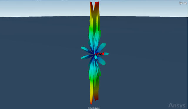
lead aircraft radar cross section
The chase aircraft is set up with two sensors. The one sensor (Servo) is used for the radar that is tracking the lead aircraft. The other sensor (Radar FOR) is notional and models the elevation and azimuth
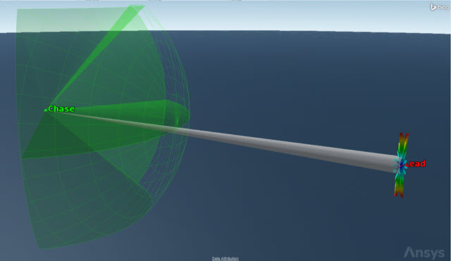
Notional view — chase aircraft servo and field of regard
The radar, simulated using the STK software's Radar capability, is a monostatic
Using the Air Rendezvous Simulation tool
The
Opening the Air Rendezvous Simulation Tool
The Air Rendezvous Simulation Tool can be found in the Aircraft Plugins menu.
- Right-click on Chase (
 ) in the Object Browser.
 - Select Aircraft Plugins in the shortcut menu.
- Select Air Rendezvous Simulation (
 ) in the Aircraft Plugins submenu.
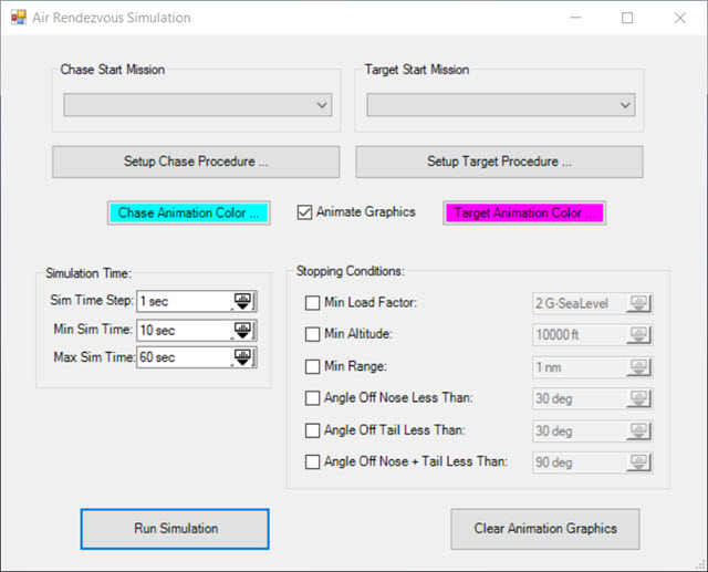
Air Rendezvous simulation tool
You can also access the Air Rendezvous Simulation tool by clicking Air Rendezvous Simulation (![]() ) on the Aviator Ui Plugins toolbar (
) on the Aviator Ui Plugins toolbar ( ). You can enable the toolbar by selecting Toolbars in the View menu, then selecting Aviator Ui Plugins in the Toolbars submenu.
Selecting the Chase and Target aircraft
The simulation involves two Aviator aircraft: the chase aircraft and the target aircraft. Start by selecting the aircraft that you want to simulate for each role.
- Open the drop-down list in the Chase Start Mission panel when the Air Rendezvous Simulation Tool opens.
- Select Chase.
- Open the drop-down list in the Target Start Mission panel.
- Select Lead.
Setting the first chase procedure
Once you have selected the aircraft, define a basic maneuver strategy for each of them. These strategies model the flight of each aircraft during the simulation. You can use any basic maneuver strategy, but at least one of the two aircraft must be using a programmatic dynamic strategy. The
- Click .
- Ensure the Horizontal / Navigation tab is selected when the Chase Simulation Procedure dialog box opens.
- Open the Strategy drop-down list.
- Select MATLAB - 3D Guidance.
- Notice that Lead is the default selection in the Target field.
- Note that the FlightTest3DGuidance MATLAB function is listed in the MFunction field in the Guidance Law panel.
- Ensure the Fuel State check box is selected in the Basic Stop Conditions panel.
- Clear the Time of Flight and Downrange check boxes.
- Click to confirm your changes and to close the Chase Simulation Procedure dialog box.
The MATLAB application will open and run in the background when you make this selection. The MATLAB Command Window will remain open in the background whenever the scenario is open.
You can click to open and view the FlightTest3DGuidance.m function and its inputs and outputs in the MATLAB Editor window. The function file, along with the functions used with other MATLAB programmatic dynamic strategies, can be found in <Install Dir>\bin\Matlab.
Each maneuver requires at least one stopping condition, which dictates when the maneuver will end regardless of whether any other goals are met. You can define more than one stopping condition if you want, and the simulation stops if any one of them is met. The Fuel State stopping condition specifies a minimum amount of fuel remaining before the aircraft will stop the maneuver.
For all procedures in this tutorial, you must clear the Time of Flight and Downrange check boxes in the Basic Stop Conditions panel. Doing this allows you to set a simulation time that doesn't conflict with Time of Flight and Downrange values. The only stopping condition you will use throughout is Fuel State, which defaults to zero pounds (0 lb) of fuel. If you don't do this, Aviator will throw an error message when you run the simulation. If this happens, go back into the procedure and ensure that the only basic stop condition selected is Fuel State.
Setting the first target procedure
The target aircraft will fly straight throughout the simulation using a Straight Ahead Horizontal / Navigation strategy. A
- Click .
- Ensure the Horizontal / Navigation tab is selected when the Target Simulation Procedure dialog box opens.
- Notice that Straight Ahead is the default Strategy setting.
- Clear the Time of Flight and Downrange check boxes in the Basic Stop Conditions panel.
- Click to confirm your changes and to close the Target Simulation Procedure dialog box.
Running the simulation
Each time you run the simulation, you create a new procedure for each aircraft. The selected procedures you create will run based on your simulation time input. These procedures are then added to the Aircraft objects' properties. You will be able to view the procedures in the 3D Graphics window. You must keep the Air Rendezvous Simulation tool open until you're finished designing all the required procedures for the mission. After you finish, you will be able to view the procedures in each aircraft's
- Enter 30 sec in the Max Sim Time field in the Simulation Time panel.
- Click .
- Click to close the PostSimulationResults window.
The Simulation Time properties affect the duration of the simulation and the frequency of sampling. The Max Sim time is the maximum duration of the simulation. If none of the selected stopping conditions are satisfied, then the simulation will end as soon as this duration has passed.
A progress window is displayed while the simulation is calculated. When the simulation completes, the progress window automatically disappears and the Post Simulation Results window appears.
Maneuvering the chase aircraft behind the lead aircraft
Use a
- Click .
- Ensure the Horizontal / Navigation tab is selected when the Chase Simulation Procedure dialog box opens.
- Open the Strategy drop-down list.
- Select Relative Bearing.
- Keep the default setting of 0 deg in the Rel Bearing field.
- Select the Fuel State check box in the Basic Stop Conditions panel.
- Clear the Time of Flight check box.
- Click twice to confirm your changes and to close the Chase Simulation Procedure dialog box.
Setting the lead stop condition
Ensure that the only basic stop condition selected is Fuel State.
- Click .
- Select the Fuel State check box in the Basic Stop Conditions panel when the Target Simulation Procedure dialog box opens.
- Clear the Time of Flight check box.
- Click to confirm your changes and to close the Target Simulation Procedure dialog box.
Running the simulation
Set the stopping conditions for the simulation.
- Enter 360 sec in the Max Sim Time field in the Simulation Time panel.
- Select the Angle Off Tail Less Than check box in the Stopping Conditions panel.
- Enter 0.1 deg in the Angle Off Tail Less Than field.
- Click .
- Click to close the PostSimulationResults window.
The simulation will stop when the angle from the body negative X axis and a vector to the other aircraft is less than this value.
Maneuvering to the right side of the lead aircraft
The chase aircraft is behind the lead aircraft. Now, it will fly to the lead aircraft's right side.
- Click .
- Ensure the Horizontal / Navigation tab is selected when the Chase Simulation Procedure dialog box opens.
- Keep the Relative Bearing strategy.
- Enter -90 deg Rel Bearing field.
- Select the Fuel State check box in the Basic Stop Conditions panel.
- Clear the Time of Flight check box.
- Click to confirm your changes and to close the Chase Simulation Procedure dialog box.
Changing the lead aircraft's Vertical / Profile strategy
Update the lead aircraft's Vertical / Profile strategy to slow the aircraft down while maintaining its Straight Ahead Horizontal / Navigation strategy.
- Click .
- Select the Vertical / Profile tab when the Target Simulation Procedure dialog box opens.
- Select the Fuel State check box in the Basic Stop Conditions panel.
- Clear the Time of Flight check box.
- Open the Maintain current airspeed drop-down list in the Airspeed panel.
- Select Decelerate at:.
- Keep the Acceleration performance model value selection.
- Click to confirm your changes and to close the Target Simulation Procedure dialog box.
Running the simulation
Set a 120-second Max Sim Time stopping condition and run the simulation.
- Enter 120 sec in the Max Sim Time field in the Simulation Time panel.
- Clear the Angle Off Tail Less Than check box in the Stopping Conditions panel.
- Click .
- Click to close the PostSimulationResults window.
Bringing the chase aircraft behind the lead aircraft
Slowing down the lead aircraft while the chase aircraft performed its turn will allow the chase aircraft to maneuver back in behind it.
- Click .
- Ensure the Horizontal / Navigation tab is selected when the Chase Simulation Procedure dialog box opens.
- Enter 0 deg in the Rel Bearing field.
- Select the Fuel State check box in the Basic Stop Conditions panel.
- Clear the Time of Flight check box.
- Click to confirm your changes and to close the Chase Simulation Procedure dialog box.
Changing the lead aircraft's Vertical / Profile strategy
The lead aircraft will maintain a Straight Ahead Horizontal / Navigation strategy but will accelerate to and maintain its maximum cruise airspeed.
- Click .
- Select the Vertical / Profile tab when the Target Simulation Procedure dialog box opens.
- Select the Fuel State check box in the Basic Stop Conditions panel.
- Clear the Time of Flight check box.
- Open the Decelerate At drop-down list in the Airspeed panel.
- Select Maintain max cruise airspeed.
- Click to confirm your changes and to close the Target Simulation Procedure dialog box.
Running the simulation
Set the stopping conditions for the simulation and run the simulation.
- Enter 360 sec in the Max Sim Time field in the Simulation Time panel.
- Select the Angle Off Tail Less Than check box in the Stopping Conditions panel.
- Enter 1.0 deg in the Angle Off Tail Less Than field.
- Click .
- Click to close the PostSimulationResults window.
Pushing the chase aircraft into a descent
Push the chase aircraft into a descent using a Push / Pull profile segment. The
- Click .
- Select the Vertical / Profile tab when the Chase Simulation Procedure dialog box opens.
- Open the Strategy drop-down list.
- Select Profile Segment – Push/Pull.
Setting the chase aircraft's descent angle
The goal of the Push/Pull Profile segment is a 15-degree angle of descent.
- Open the Pull Up drop-down list.
- Select Push Over.
- Enter -15 deg in the Flight Path Angle is field in the Stop When panel.
- Select the Fuel State check box in the Basic Stop Conditions panel.
- Clear the Time of Flight check box.
- Click .
- Click to set a valid G-SeaLevel setting and to close the PushPullG invalid value and Chase Simulation Procedure dialog boxes.
Stop When options are used to define conditions that will cause the aircraft to stop the maneuver whenever a condition is met.
Push over G is constrained by the initial and / or stop flight path angle. Clicking automatically sets a valid G-SeaLevel value.
Setting the lead stop condition
The lead aircraft will continue to fly straight ahead.
- Click .
- Select the Fuel State check box in the Basic Stop Conditions panel when the Target Simulation Procedure dialog box opens.
- Clear the Time of Flight check box.
- Click to confirm your changes and to close the Target Simulation Procedure dialog box.
Running the simulation
Set a 60-second Max Sim Time stopping condition and run the simulation.
- Enter 60 sec in the Max Sim Time field in the Simulation Time panel.
- Clear the Angle Off Tail Less Than check box in the Stopping Conditions panel.
- Click .
- Click to close the PostSimulationResults window.
Lowering the chase aircraft's altitude
Use an Autopilot - Vertical Plane strategy to lower the chase aircraft's altitude. The
- Click .
- Select the Vertical / Profile tab when the Chase Simulation Procedure dialog box opens.
- Open the Strategy drop-down list.
- Select Autopilot – Vertical Plane.
- Open the Mode drop-down list in the Altitude panel.
- Select Hold Initial Altitude Rate.
- Select the Fuel State check box in the Basic Stop Conditions panel.
- Clear the Time of Flight check box.
- Click to confirm your changes and to close the Chase Simulation Procedure dialog box.
The aircraft will attempt to hold the altitude rate at which it began the maneuver.
Setting the lead stop condition
The lead aircraft will continue to fly straight ahead.
- Click .
- Select the Fuel State check box in the Basic Stop Conditions panel when the Target Simulation Procedure dialog box opens.
- Clear the Time of Flight check box.
- Click to confirm your changes and to close the Target Simulation Procedure dialog box.
Running the simulation
Set a 15,000-foot minimum altitude stopping condition for the simulation.
- Keep 60 sec in the Max Sim Time field in the Simulation Time panel.
- Select the Min Altitude check box in the Stopping Conditions panel.
- Enter 15000 ft Min Altitude field.
- Click .
- Click to close the PostSimulationResults window.
The simulation will stop once either aircraft drops below this altitude.
Leveling the chase aircraft at 10,000 feet
The chase aircraft will descend to 10,000 feet and level off.
- Click .
- Select the Vertical / Profile tab when the Chase Simulation Procedure dialog box opens.
- Open the Mode drop-down list in the Altitude panel.
- Select Specify Altitude.
- Keep the default value of 10000 ft in the Absolute Altitude field.
- Enter 20000 ft/min in the Control Altitude Rate field.
- Select the Fuel State check box in the Basic Stop Conditions panel.
- Clear the Time of Flight check box.
- Click to confirm your changes and to close the Chase Simulation Procedure dialog box.
The aircraft will attempt to maintain a specified altitude above the current ground reference.
This sets the absolute altitude that you want the aircraft to achieve.
This sets the altitude rate at which the aircraft will adjust its altitude with respect to the goal to a rapid 20,000 feet per minute.
Setting the lead stopping condition
As before, the lead aircraft will continue to fly straight ahead.
- Click .
- Select the Fuel State check box in the Basic Stop Conditions panel when the Target Simulation Procedure dialog box opens.
- Clear the Time of Flight check box.
- Click to confirm your changes and to close the Target Simulation Procedure dialog box.
Running the simulation
Clear the minimum altitude stopping condition so that the simulation stops after a maximum of 60 seconds.
- Keep 60 sec in the Max Sim Time field in the Simulation Time panel.
- Clear the Min Altitude check box in the Stopping Conditions panel.
- Click .
- Click to close the PostSimulationResults window.
Ascending above the lead aircraft
The chase aircraft will climb to an altitude of 40,000 feet.
- Click .
- Select the Vertical / Profile tab when the Chase Simulation Procedure dialog box opens.
- Enter 40000 ft in the Absolute Altitude field in the Altitude panel.
- Select the Fuel State check box in the Basic Stop Conditions panel.
- Clear the Time of Flight check box.
- Click to confirm your changes and to close the Chase Simulation Procedure dialog box.
Setting the lead stop condition
The lead aircraft will continue to fly straight ahead.
- Click .
- Select the Fuel State check box in the Basic Stop Conditions panel when the Target Simulation Procedure dialog box opens.
- Clear the Time of Flight check box.
- Click to confirm your changes and to close the Target Simulation Procedure dialog box.
Running the simulation
Set the Max Sim Time stopping condition to 120 seconds and run the simulation.
- Enter 120 sec in the Max Sim Time field in the Simulation Time panel.
- Click .
- Click to close the PostSimulationResults window.
Descending back to the lead aircraft's altitude
Finally, the chase aircraft will descend back down to 25,000 feet and fall in behind the lead aircraft.
- Click .
- Select the Vertical / Profile tab when the Chase Simulation Procedure dialog box opens.
- Enter 25000 ft in the Absolute Altitude field in the Altitude panel.
- Select the Fuel State check box in the Basic Stop Conditions panel.
- Clear the Time of Flight check box.
- Click to confirm your changes and to close the Chase Simulation Procedure dialog box.
Setting the lead stop condition
The lead aircraft will continue to fly straight ahead.
- Click .
- Select the Fuel State check box in the Basic Stop Conditions panel when the Target Simulation Procedure dialog box opens.
- Clear the Time of Flight check box.
- Click to confirm your changes and to close the Target Simulation Procedure dialog box.
Running the simulation
Keep the simulation set to stop running after a maximum of 120 seconds.
- Keep 120 sec in the Max Sim Time field in the Simulation Time panel.
- Click .
- Click to close the PostSimulationResults window.
- Exit out of the Air Rendezvous Simulation Tool.
Viewing the chase and lead aircraft flight routes
You can view the flight routes of both aircraft in the 3D Graphics window.
- Bring the 3D Graphics window to the front.
- Use your mouse to set your view so that you can see both aircraft's routes.
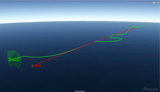
3D view of chase and lead
- Right-click on Chase () in the Object Browser.
- Select Zoom To in the shortcut menu.
- Click Increase Time Step (
 ) in the Animation toolbar to set the X Real Time Multiplier to 32.00.
 - Click Start (
 ) to animate your scenario.
 - Follow the Chase aircraft as it maneuvers around Lead based on your procedure inputs.
- Click Reset (
 ) when you are finished animating the scenario.
Notice how the Servo sensor tracks Lead when it is able, based on its preset angular constraints.
![]()
Servo tracking lead
Creating custom graphs to analyze the radar as it tracks the lead aircraft
You have designed the flight routes of both the chase and lead aircraft. Now it's time to analyze the chase aircraft radar's ability to track the lead aircraft.
Calculating access between the lead aircraft and the Radar object
Start by calculating the access intervals between the lead aircraft and the radar attached to the chase aircraft.
- Right-click on Lead () in the Object Browser.
- Select Access... (
 ) in the shortcut menu.
 - Expand (
 ) Chase () in the Associated Objects list when the Access tool opens.
 - Expand () Servo (
 ).
). - Select Radar (
 ).
). - Click
 in the Access toolbar.
 - Click below the Reports panel.
Creating a custom graph of the RCS, azimuth, and elevation over time
Create a graph of the RCS (radar cross section), Azimuth, and Elevation over time.
- Select the My Styles (
 ) folder in the Styles panel list when the Report & Graph Manager opens.
 - Click Create new graph style (
 ) in the Styles panel toolbar.
 - Enter AzEl RCS while in rename mode.
- Select the Enter key.
Selecting the data providers, groups and elements
Select the data providers, groups and elements needed in your custom graph.
- Select the Content page when the Properties Browser opens.
- Expand () the AER Data (
 ) data provider in the data provider list.
 - Expand () the Default () data provider group.
- Azimuth (
 )
) - Elevation ()
- Azimuth (
- Click Insert Y2 Axis (
 ) in the Y2 Axis panel.
 - Expand () the Radar RCS () data provider.
- Select the RCS () data provider element.
- Click Insert Y Axis () in the Y Axis panel.
- Click to confirm your selections and to close the Properties Browser.
Creating a custom graph of the RCS and range over time
Create a graph of the RCS and the range over time.
- Select AzEl RCS (
 ) in the My Styles () folder in the Styles panel list.
 - Click Duplicate (
 ) in the Styles panel toolbar.
 - Ensure the Content page is selected when the Properties Browser opens.
- Select both AER Data-Default-Azimuth and AER Data-Default-Elevation in the Y2 Axis panel.
- Click Remove Y2 Axis (
 ).
). - Expand () the AER Data () data provider.
- Expand () the Default () data provider group.
- Select the Range () data provider element.
- Click Insert Y2 Axis () in the Y2 Axis panel.
Changing the graph's units of measure
Change the graph units of measure for the Range data provider element from kilometers to nautical miles.
- Select AER Data-Default-Range in the Y2 Axis panel.
- Click .
- Clear the Use Defaults check box when the Units: AER Data-Default-Range dialog box opens.
- Select Nautical Miles (nm) in the New Unit Value list.
- Click to confirm your changes and to close the Units: AER Data-Default-Range dialog box.
- Click to confirm your changes and to close the Properties Browser.
Renaming the new graph
Rename the graph Range RCS.
- Right-click on the AzEl RCS (2) () graph in the My Styles () folder in the Styles panel list.
- Select Rename in the shortcut menu.
- Rename AzEl RCS (2) () Range RCS.
Creating a custom graph of the SNR and range over time
Create a graph of the SNR and the range over time by duplicating the Range RCS graph. SNR is the signal-to-noise ratio.
- Select Range RCS () in the My Styles () folder in the Styles panel list.
- Click Duplicate () in the Styles panel toolbar.
- Ensure the Content page is selected page when the Properties Browser opens.
- Select Radar RCS-RCS in the Y Axis panel.
- Click Remove Y Axis ().
- Expand () the Radar SearchTrack () data provider.
- Select the S/T Integrated SNR () data provider element.
- Click Insert Y Axis () in the Y Axis panel.
- Click to confirm your changes and to close the Properties Browser.
Renaming the new graph
Rename the graph Range SNR.
- Right-click on the AzEl RCS (2) () graph in the My Styles () folder in the Styles panel list.
- Select Rename in the shortcut menu.
- Rename AzEl RCS (2) () Range SNR.
Creating a custom graph of the SNR, azimuth and elevation over time
Create a graph of the SNR, azimuth, and the elevation over time by duplicating the Range SNR graph you just created.
- Select Range SNR () in the My Styles () folder in the Styles panel list.
- Click Duplicate () in the Styles panel toolbar.
- Ensure the Content page is selected when the Properties Browser opens.
- Select AER Data-Default-Range in the Y2 Axis panel.
- Click Remove Y2 Axis ().
- Expand () the AER Data () data provider.
- Expand () the Default () data provider group.
- Multi-select the following data provider elements:
- Azimuth ()
- Elevation ()
- Azimuth (
- Click Insert Y2 Axis () in the Y2 Axis panel.
- Click to confirm your changes and to close the Properties Browser.
Renaming the new graph
Rename the graph AzEl SNR.
- Right-click on the AzEl SNR (2) () graph in the My Styles () folder in the Styles panel list.
- Select Rename in the shortcut menu.
- Rename AzEl SNR (2) () AzEl SNR.
Analyzing the custom graphs
You can generate all four custom graphs at the same time, analyze the data and compare the graphs to the data display that you placed on the 3D Graphics window.
- Bring the Report & Graph Manager back to the front.
- Multi-select your four custom graphs () in the My Styles () folder.
- Click .
- View the graphs to see the ranges of Azimuth, Elevation, and Range tested and how they affect the detected RCS and S/N values.
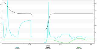
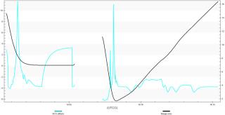
RCS - Azimuth - Elevation and graph RCS - Range graph
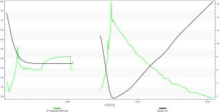
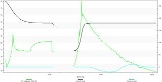
S/T Integrated SNR - Range graph and S/T Integrated SNR - Azimuth - Elevation graph
Creating a display of dynamic data
The
Creating a custom radar data display report
Create a custom report that you will use for a dynamic display of the radar data in the 3D Graphics window.
- Return to the Report & Graph Manager.
- Select the My Styles () folder in the Styles panel list of the Report & Graph Manager.
- Click Create new report style (
 ) in the Styles panel toolbar.
 - Enter Radar Data Display while in rename mode.
- Select the Enter key.
Selecting the AER data providers elements
Select the AER data provider elements needed in your custom report.
- Ensure the Content page is selected when the Properties Browser opens.
- Expand () the AER Data () data provider.
- Expand () the Default () data provider group.
- Multi-select the following data provider elements:
- Time ()
- Azimuth ()
- Elevation ()
- Range ()
- Click Insert ().
Selecting the Radar RCS and SearchTrack data providers elements
Select the Radar RCS and Radar SearchTrack data provider elements needed in your custom report.
- Expand () the Radar RCS () data provider.
- Select the RCS () data provider element.
- Click Insert ().
- Expand () the Radar SearchTrack () data provider.
- Select the S/T Integrated SNR () data provider element.
- Click Insert ().
- Click to confirm your selections and to close the Properties Browser.
Adding the custom report to the 3D Graphics window
Use the 3D Graphics Displays option in the Access tool to select the Radar Data Display report for dynamic display in the 3D Graphics window.
- Bring the Access tool to the front.
- Click .
- Click when the 3D Graphics Data Display dialog box opens.
- Select Radar Data Display in the Styles list when the Add a Data Display dialog box opens.
- Click to confirm your selection and to close the Add a Data Display dialog box.
- Click to confirm your selection and to close the 3D Graphics Data Display dialog box.
Comparing the graph data to the data display in the 3D Graphics window
You can compare the graph analysis to the data display and the visual representation of the aircraft in the 3D Graphics window. This is a good way to obtain situational awareness of your mission.
Viewing the point of peak SNR
View the point in your simulation when the Search / Track Signal-to-Noise ratio is greatest.
- Bring the AzEl SNR graph to the front.
- Right-click on the S/T Integrated SNR peak.
- Select Set Animation Time in the shortcut menu.
- Bring the 3D Graphics window to the front.
- Right-click on Chase () in the Object Browser.
- Select Zoom To in the shortcut menu.
- Use your mouse to set the view so that you can see both the Chase and the Lead aircraft.
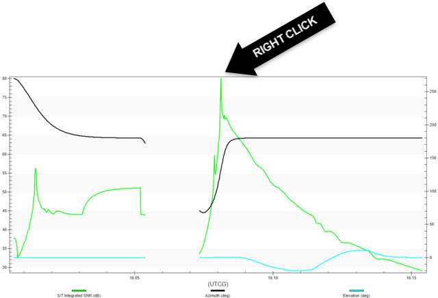
S/T Integrated SNR peak
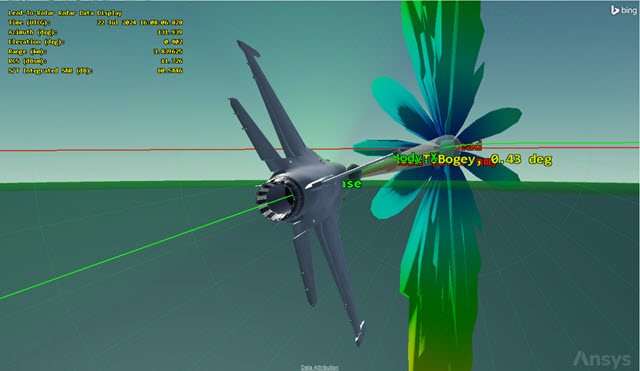
chase radar — peak SNR
The data display shows the information you created in the custom Radar Data Display report.
Viewing the interval when no SNR data is gathered
Your graphs show a gap where no SNR data is collected by the Chase aircraft's radar. View that portion of the simulation in the 3D Graphics window to understand why.
- Return to the AzEl SNR graph.
- Right-click on the graph where there is no data for S/T Integrated SNR.
- Select Set Animation Time in the shortcut menu.
- Bring the 3D Graphics window to the front.
- Use your mouse to set the view so that you can see both the Chase and Lead aircraft.
- Zoom out until you can see the RadarFOR sensor's field of view.
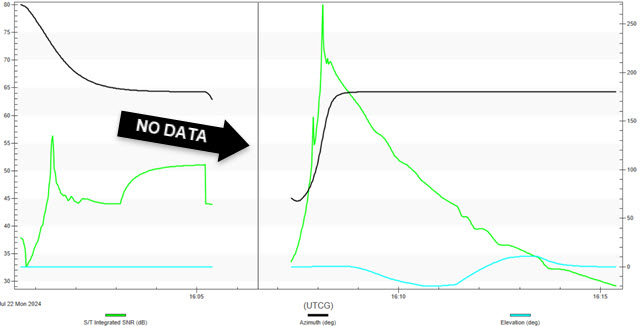
S/T Integrated SNR — no data
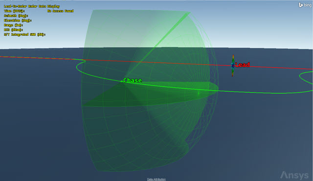
Chase radar — no access
This view shows when the radar on the chase aircraft can't access the lead aircraft. It shows that the radar is restricted to RadarFOR's field of regard and therefore there's no access.
Saving your work
Clean up your workspace and close out your scenario.
- Close all open reports, graphs, and tools except 3D Graphics window.
- Save (
 ) your work.
 - Close the scenario when finished.
Summary
You used the STK application's core capabilities and the Aviator Pro capability's Air Rendezvous Simulation Tool to create specialized stopping conditions to feed Aviator maneuvers to a lead and a chase aircraft. You added multiple basic procedures to the aircraft flying in the lead position while the chase aircraft rendezvoused with the lead aircraft. You simultaneously created procedures for the chase aircraft to maneuver it behind, around, below and above the lead aircraft, finally leveling off behind the lead aircraft. The chase aircraft had a radar system that tracked off its nose from ±60 degrees azimuth and ±45 degrees elevation. The lead aircraft had a notional radar cross section. After creating the simulation you collected radar statistics and obtained situational awareness of the rendezvous and radar run in the 3D Graphics window.