Part 12:
STK Pro, STK Premium (Air), STK Premium (Space), or STK Enterprise
You can obtain the necessary licenses for this tutorial by contacting AGI Support at support@agi.com or 1-800-924-7244.
The results of the tutorial may vary depending on the user settings and data enabled (online operations, terrain server, dynamic Earth data, etc.). It is acceptable to have different results.
This lesson requires STK 12.9 or newer to complete.
Capabilities covered
This lesson covers the following STK Capabilities:
- STK Pro
- Radar
Problem statement
Engineers and operators need to determine how various radar settings will affect its ability to track different sized targets. They want to know how the following settings affect a radar's ability to track multiple target types:
- Radar Cross Section
- Pulse Repetition Frequency
- Gain
- Pulse integration
Solution
Use STK Pro and STK's Radar capability to:
- Create an airfield radar site
- Model an airport surveillance radar
- Build a monostatic radar
- Test various settings against multiple targets
- Determine probability of detection
What you will learn
Upon completion of this tutorial, you will understand:
- Radar Cross Sections
- Monostatic Radars and their settings
- Radar Data Providers
Video guidance
Watch the following video. Then follow the steps below, which incorporate the systems and missions you work on (sample inputs provided).
Creating a new scenario
Create a new scenario.
- Launch STK (
 ).
). - Click
 Create a Scenario in the Welcome to STK dialog box.
 - Enter the following in the New Scenario Wizard:
- When finished, click .
- When the scenario loads, click Save (
 ). A folder with the same name as your scenario is created for you in the location specified above.
 - Verify the scenario name and location in the Save As window.
- Click .
| Option | Value |
|---|---|
| Name | STK_Radar |
| Location | Default |
| Start | Default day, month and year. Set the time to 03:00:00.000 UTCG |
| Stop | +30 min |
Save (![]() ) often!
) often!
Turning off Terrain Server
This is an introduction to Radar. Terrain will not be used in this analysis.
- Right click on STK_Radar () in the Object Browser.
- Select Properties (
 ) in the shortcut menu.
 - Select the Basic - Terrain page when the Properties Browser opens.
- Clear the Use terrain server for analysis check box.
- Click to accept the changes and close the Properties Browser.
Turning on Label Declutter
Turn on Label Declutter to reposition object labels so they do not obstruct one another while in close proximity.
- Bring the 3D Graphics window to the front.
- Click Properties (
 ) in the 3D Window Defaults toolbar.
 - Select the Details page when the Properties Browser opens.
- Select the Enable check box in the Label Declutter panel.
- Click to accept changes and close the Properties Browser.
Inserting the target aircraft
Insert an Aircraft (![]() ) object. We will use the aircraft to analyze the airfield surveillance radar.
) object. We will use the aircraft to analyze the airfield surveillance radar.
- Select Aircraft (
 ) in the Insert STK Objects tool.
 - Select the Insert Default () method.
- Click .
- Right-click on Aircraft1 () in the Object Browser.
- Select Rename in the shortcut menu.
- Rename the Aircraft1 () to Target_Acft.
Creating the target aircraft's flight route
Create Target_Acft's (![]() ) route, then modify it's altitude and speed.
) route, then modify it's altitude and speed.
- Open Target_Acft's () properties ().
- Select the Basic - Route page when the Properties Browser opens.
- Click two times.
- Set the following:
- Click .
- Select the Altitude: and Speed: check boxes in the Set All Grid Values dialog box.
- Set the following:
- Click to close the Set All Grid Values dialog box.
- Click to accept the changes and keep the Properties Browser open.
| Waypoint | Latitude | Longitude |
|---|---|---|
| One | 37 deg | 139.7 deg |
| Two | 34 deg | 139.1 deg |
| Option | Value |
|---|---|
| Altitude | 25000 ft |
| Speed | 330 mi/hr |
Changing the target aircraft's 3D model
You can select a realistic 3D model for your Aircraft (![]() ) object.
) object.
- Select the 3D Graphics - Model page.
- Click the Model File: ellipsis (
 ).
). - Select c-130_hercules.glb in the File dialog box.
- Click .
- Click to accept the changes and keep the Properties Browser open.
Specifying the radar cross section
Before setting up and constraining a radar system, Radar allows you to specify an important property of a potential radar target - its radar cross section (RCS). Use the RCS of a popular four-engined turboprop transport aircraft.
- Select the RF - Radar Cross Section page.
- Clear the Inherit check box.
- Enter 19 dBsm (decibels referenced to a square meter) in the Constant RCS Value: field.
- Click to accept the changes and keep the Properties Browser open.
This allows you to set the RCS settings for the Aircraft (![]() ) object instead of inheriting the settings from the Scenario (
) object instead of inheriting the settings from the Scenario (![]() ) object.
) object.
Ideally, you would want to use an Aspect Dependent RCS file. Since you don't have one, you will use a constant value. The constant value we set is the RCS of a sphere that radiates isotropically.
Displaying radar cross section graphics
The 3D Graphics RCS page allows you to control the 3D display of Radar Cross Section contour lines.
- Select the 3D Graphics - Radar Cross Section page.
- Select the Show Volume check box in the Volume Graphics panel.
- Click to accept the changes and close the Properties Browser.
- Bring the 3D Graphics window to the front.
- Right-click on Target_Acft () in the Object Browser.
- Select Zoom To in the shortcut menu.
- Use your mouse to zoom out until you can see the RCS sphere.
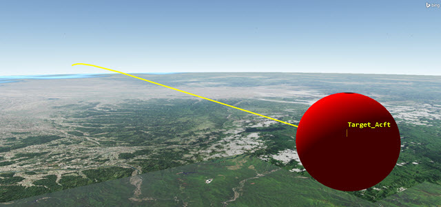
Radar Cross Section Sphere
Inserting the radar site
Use a Place (![]() ) object as the radar site location.
) object as the radar site location.
- Insert a Place (
 ) object using the Insert Default () method.
 - Rename Place1 (
 ) to Radar_Site.
Defining the radar site's location
Define the location of Radar_Site (![]() ) and raise its height above ground 50 ft to model the radar antenna height.
) and raise its height above ground 50 ft to model the radar antenna height.
- Open Radar_Site's () properties ().
- Select the Basic - Position page when the Properties Browser opens.
- Set the following in the Position panel:
- Click to accept the changes and close the Properties Browser.
- Bring the 3D Graphics window to the front.
- Zoom To Radar_Site ().
- Use your mouse to obtain situational awareness of the radar site's location.
| Option | Value |
|---|---|
| Latitude | 35.75174 deg |
| Longitude | 139.35621 deg |
| Height Above Ground | 50 ft |
Raising the Place (![]() ) object 50 feet above the ground simulates the height of the radar antenna.
) object 50 feet above the ground simulates the height of the radar antenna.

Radar Site
Inserting the antenna servo system
Insert a Sensor (![]() ) object to simulate a servo system for antenna positioning. In STK, you could create a spinning sensor to simulate a spinning radar antenna normally seen at an airfield. However, you will lock the sensor onto the aircraft and constrain the sensor to point in a limited area. This simulates the actual field of view of the airfield surveillance radar both horizontally and vertically.
) object to simulate a servo system for antenna positioning. In STK, you could create a spinning sensor to simulate a spinning radar antenna normally seen at an airfield. However, you will lock the sensor onto the aircraft and constrain the sensor to point in a limited area. This simulates the actual field of view of the airfield surveillance radar both horizontally and vertically.
- Insert a Sensor (
 ) object using the Insert Default () method.
 - Select Radar_Site () in the Select Object dialog box.
- Click .
- Rename Sensor1 () to Servo_System.
Defining the sensor field of view
Define Servo_System's (![]() ) field of view using a Simple Conic sensor pattern. You will use the sensor's field of view for situational awareness when Servo_System(
) field of view using a Simple Conic sensor pattern. You will use the sensor's field of view for situational awareness when Servo_System(![]() ) points the antenna at Target_Acft (
) points the antenna at Target_Acft (![]() ).
).
- Open Servo_System's () properties ().
- Select the Basic - Definition page when the Properties Browser opens.
- Enter 2 deg in the Cone Half Angle: field in the Simple Conic panel.
- Click to accept the changes and keep the Properties Browser open.
Targeting the aircraft
Use the Targeted pointing type to point Servo_System (![]() ) to Target_Acft(
) to Target_Acft(![]() ).
).
- Select the Basic - Pointing page.
- Open the Pointing Type: shortcut menu.
- Select Targeted.
- Move (
 ) Target_Acft () from the Available Targets list to the Assigned Targets list.
 - Click to accept the changes and keep the Properties Browser open.
Setting range and elevation angle constraints
There are many types of radar systems. A typical airport surveillance radar's nominal range is 60 miles and the elevation angle of the beam can track from 0 to 30 degrees. Anything higher than 30 degrees is the cone of silence in which the radar cannot track the aircraft. Extend the Servo_System's (![]() ) maximum range further than 60 miles in order to lock onto the aircraft when it's above the horizon.
) maximum range further than 60 miles in order to lock onto the aircraft when it's above the horizon.
Adding the range and elevation constraints
Add range and elevation angle to the Active Constraints list.
- Select the Constraints - Active page.
- Click Add new constraints (
 ) in the Active Constraints toolbar.
 - Using the Ctrl key on your keyboard, select the following in the Constraint Name list in the Select Constraints to Add dialog box:
- Elevation Angle
- Range
- Click .
- Click to close the Select Constraints to Add dialog box.
Setting the max values
Set the max values for range and elevation angle constraints.
- Select Elevation Angle in the Active Constraints list.
- Select the Max: check box in the Constraint Properties - Elevation Angle panel.
- Enter 30 deg in the Max: field.
- Select Range in the Active Constraints list.
- Select the Max: check box in the Constraint Properties - Range panel.
- Enter 150 km in the Max: field.
- Click to accept the changes and close the Properties Browser.
Generating an azimuth elevation range report
Generate an azimuth-elevation-range (AER) report to see what affect your constraints have on your accesses.
- Right click on Servo_System (
 ) in the Object Browser.
 - Select Access... (
 ) in the shortcut menu.
 - Select Target_Acft () in the Associated Objects list when the Access Tool opens.
- Click
 .
. - Click in the Reports panel.
- Look at the Elevation (deg) column.
- Notice that the first access ends and the second access begins at an approximate elevation angle of 30 degrees.
- Close the AER report. and the Access Tool when finished.
There is a break in access when the elevation angle exceeds 30 degrees due to the modeled cone of silence.
Looking at the sensor's field of view
Animate through the scenario to get a visual idea of when Servo_System (![]() ) tracks Target_Acft (
) tracks Target_Acft (![]() ).
).
- Bring the 3D Graphics window to the front.
- Click Reset (
 ) in the Animation Toolbar.
 - Right-click on Radar_Site ().
- Select Zoom To.
- Use your mouse to zoom out until you can see the entire aircraft flight route, the radar site, and the sensor's field of view.
- Click Decrease Time Step (
 ) in the Animation Toolbar until Time Step: is 1.00 sec.
 - Click Start (
 ) in the Animation Toolbar to animate the scenario.
 - Watch the animation. You can see the sensor turn off when the elevation angle exceeds 30 degrees, and turn back on when it returns to 30 degrees.
- Click Reset () in the Animation Toolbar when finished.
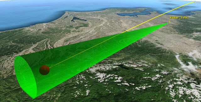
Sensor Field of View
Inserting an airport surveillance radar
Insert a Radar (![]() ) object to create an airport surveillance radar. We will model actual airport surveillance radar specifications that are easily available to the public.
) object to create an airport surveillance radar. We will model actual airport surveillance radar specifications that are easily available to the public.
- Insert a Radar (
 ) object using the Insert Default () method.
 - Select Servo_System () in the Select Object dialog box.
- Click .
- Rename Radar1 () to ASR.
Modeling a monostatic radar
Model a Monostatic radar with a Search/Track mode. This will model a common antenna for both transmitting and receiving, and detect and track point targets.
To understand constants and equations used in STK, look at Search/Track Radar Constants and Equations in STK Help.
- Open ASR's () properties ().
- Select the Basic - Definition page when the Properties Browser opens.
- Notice that Radar System defaults to Monostatic.
- Select the Mode tab.
- Notice that Radar Monostatic Mode defaults to Search Track.
Defining the waveform
The waveform in your system will use a fixed pulse repetition frequency (PRF), with a PRF of ~1000 Hz. Radar systems often use multiple pulse integration to increase the signal-to-noise ratio. The PRF is the number of pulses of a repeating signal in a specific time unit. After producing a brief transmission pulse, the transmitter is turned off in order for the receiver to hear the reflections of that signal off of targets.
- Select the Waveform sub-tab.
- Notice that Waveform defaults to Fixed PRF.
- Select the Pulse Definition sub-sub-tab.
- Notice that the PRF option is selected and the default value is 0.001 MHz.
- Keep that value since your system's PRF is ~1000 Hz.
Defining the pulse width
Pulse width is the width of the transmitted pulse (the uncompressed RF bandwidth can also be taken as the inverse of the pulse width). Set the pulse width to one microsecond.
- Open the Pulse Width shortcut menu (
 ).
). - Select usec.
- Enter 1 usec in the Pulse Width field.
- Click to accept the changes and keep the Properties Browser open.
Defining the antenna model
Model the antenna using the cosine squared aperture rectangular antenna pattern. The antenna transmit frequency for this radar is between 2.7-2.9 GHz.
- Select the Antenna tab.
- Select the Model Specs sub-tab.
- Click the Antenna Model Component Selector (
 ).
). - Select Cosine Squared Aperture Rectangular (
 ) in the Antenna Models list when the Select Component dialog box opens.
 - Click to close the Select Component dialog box.
- Select the Use Beamwidth option.
- Set the following:
- Click to accept the changes and keep the Properties Browser open.
| Option | Value |
|---|---|
| X Dim Beamwidth | 5 deg |
| Y Dim Beamwidth | 1.4 deg |
| Design Frequency | 2.8 GHz |
| Main-lobe Gain | 34 dB |
| Efficiency | 55 % |
Defining the radar transmitter
The transmitter has a frequency range of 2.7-2.9 GHz, a peak power of 20 kW.
- Select the Transmitter tab.
- Select the Frequency option.
- Enter 2.8 GHz in the Frequency field.
- Enter 20 kW in the Power: field.
- Click to accept the changes and keep the Properties Browser open.
Setting the polarization
An ASR system can use linear or circular polarization. You will model linear polarization.
- Select the Polarization sub-tab.
- Select the Use check box.
- Keep the default setting of Linear.
- Click to accept the changes and keep the Properties Browser open.
Setting the radar receiver's polarization
You don't have specific values regarding the low noise amplifier settings. These would be applied on the Receiver's Specs sub-tab. However, you know the polarization and want to add the receiver's system noise temperature. Let's set the polarization model type to Linear now.
- Select the Receiver tab.
- Select the Polarization sub-tab.
- Select the Use check box
- Keep the default setting of Linear.
- Click to accept the changes and keep the Properties Browser open.
Adding the radar receiver's system noise temperature
Next, add the receiver's system noise temperature to your analysis. You will compute system noise temperature using the default values, and take into account Sun and Cosmic Background noise.
- Select the System Noise Temperature sub-tab.
- Select the Compute option.
- Select the Compute option in the Antenna Noise panel.
- Select the Sun check box.
- Select the Cosmic Background check box.
- Click to accept the changes and close the Properties Browser.
- Save () your scenario.
Determining probability of detection
You will base the probability of detection (Pdet) on a value of 0.800000 or higher, one (1) being the highest value. You will also look at signal-to-noise ratio (SNR) and pulse integration. You will start by determining the Pdet of the large turboprop aircraft. Then, you will change Target_Acft's (![]() ) constant RCS value to simulate a medium-sized aircraft, then a small-sized aircraft, and then a bird. Finally, you'll load a notional Aspect Dependent RCS file to see the difference between that and the constant value RCS sphere.
) constant RCS value to simulate a medium-sized aircraft, then a small-sized aircraft, and then a bird. Finally, you'll load a notional Aspect Dependent RCS file to see the difference between that and the constant value RCS sphere.
Computing access
Compute access between ASR (![]() ) and Target_Acft (
) and Target_Acft (![]() ).
).
- Right-click on ASR () in the Object Browser.
- Select Access... () in the shortcut menu.
- Select Target_Acft () in the Associated Objects list when the Access Tool opens.
- Click .
Generating a Radar SearchTrack report
Now that you calculated access between ASR (![]() ) and Target_Acft (
) and Target_Acft (![]() ), generate a Radar SearchTrack report.
), generate a Radar SearchTrack report.
- Click .
- Select the Radar SearchTrack report (
 ) when the Report & Graph Manager opens.
 - Click .
- Click when the report opens.
- Enter 30 sec in the Step: field.
- Press Enter on your keyboard.
Understanding the data
The content of a report or graph is generated from the selected data providers for the report or graph style. The data provider you'll focus on in this analysis is Radar SearchTrack.
Observing Pdet
Look at the difference between S/T Pdet1 and S/T Integrated Pdet in the report. S/T Pdet1 is based off of a single pulse. S/T Integrated PDet uses multiple pulses.
- Look at the first line in the report.
- Locate the two columns S/T Pdet1 and S/T Integrated Pdet.
- Note the difference in the values.
- Notice that overall tracking is good when using pulse integration (Pdet of 0.8 or higher).
- Keep the report open.
Pulse integration improves the ability of the radar to detect targets by combining the returns from multiple pulses. You can see this in the S/T Pulses Integrated column in the report.
Observing SNR
Look at the difference between S/T SNR1 (dB) and S/T Integrated SNR (dB) in the report. S/T SNR1 (dB) is based on a single pulse and S/T Integrated SNR (dB) on pulse integration.
- Locate the two columns S/T SNR1 (dB) and S/T Integrated SNR (dB).
- Note the differences in the values.
- Again, the pulse integration allows for a better SNR.
Simulating a medium-sized aircraft
Next, simulate a medium-sized aircraft.
- Open Target_Acft's () properties ().
- Select the RF - Radar Cross Section page.
- Enter 10 dBsm in the Constant RCS Value: field.
- Click to accept the changes and keep the Properties Browser open.
- Return to the Radar SearchTrack report.
- Click Refresh (F5) (
 ) in the report's toolbar.
 - Note the S/T Pdet1, S/T Integrated Pdet, S/T SNR1 (dB), and S/T Integrated SNR (dB) changes.
The radar's ability to track this aircraft has diminished due to the aircraft's smaller RCS.
Simulating a small-sized aircraft
Simulate a small sized aircraft.
- Return to Target_Acft's () properties ()..
- Enter zero (0) dBsm in the Constant RCS Value: field.
- Click to accept the changes and keep the Properties Browser open.
- Return to the Radar SearchTrack report.
- Click Refresh (F5) () in the report's toolbar.
- Note the S/T Pdet1, S/T Integrated Pdet, S/T SNR1 (dB), and S/T Integrated SNR (dB) changes.
The radar's ability to track this aircraft has again diminished due to the aircraft's smaller RCS.
Simulating birds and stealth
Simulate a bird and a large, somewhat stealthy aircraft.
- Return to Target_Acft's () properties ().
- Enter -20 dBsm in the Constant RCS Value: field.
- Click to accept the changes and keep the Properties Browser open.
- Return to the Radar SearchTrack report.
- Click Refresh (F5) () in the report's toolbar.
- Note the S/T Pdet1, S/T Integrated Pdet, S/T SNR1 (dB), and S/T Integrated SNR (dB) changes.
Looking at the results, your system might need a different frequency or more power.
Using Aspect Dependent RCS files
If you have an Aspect Dependent RCS file built for a specific target aircraft, your data will be much more realistic.
Loading an external file
Load an installed Aspect Dependent RCS file.
- Return to Target_Acft's () properties ().
- Open the Compute Type: shortcut menu.
- Select External File.
- Click the Filename: ellipsis ().
- Browse to <STK install folder>\Data\Resources\stktraining\samples\SeaRangeResources\X-47B
- Select X-47B_Notional_Sample.rcs in the Select File dialog box.
- Click .
- Click .
- Click to accept the changes and close the Properties Browser.
Visualizing the RCS pattern
View the RCS pattern in the 3D Graphics window.
- Bring the 3D Graphics window to the front.
- Zoom To Target_Acft ().
- Use your mouse to get a good view of the aspect dependent RCS pattern.
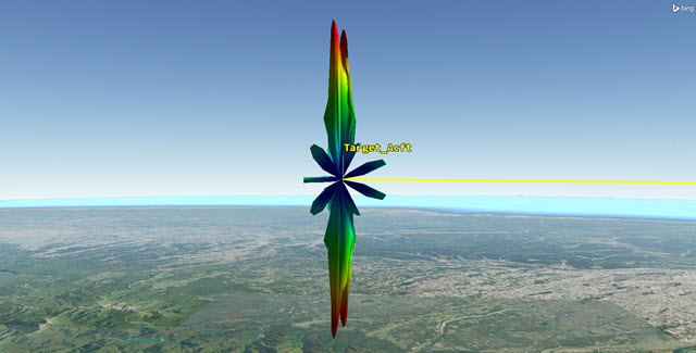
Aspect Dependent RCS Pattern
Viewing the data
Refresh the Radar SearchTrack report to see the changes in SNR, PDet and Pulse Integration.
- Return to the Radar SearchTrack report.
- Click Refresh (F5) () in the report's toolbar.
- Note the S/T Pdet1, S/T Integrated Pdet, S/T SNR1 (dB), and S/T Integrated SNR (dB) changes.
Depending on the reflection from the aircraft back to the radar, you could see fluctuation in your values. This is noticeable in the S/T Pulses Integrated column.
Viewing RCS data in a graph
Use the RCS graph style to visualize changes to RCS Decibel (dBsm). Note the cone of silence in the middle of the graph.
- Return to the Report & Graph Manager.
- Ensure the Object Type: is set to Access.
- Select Place-Radar_Site-Sensor-Servo_System-Radar-ASR-To-Aircraft-Target_Acft in the Object Type: list.
- Select the Radar RCS graph (
 ) in the Installed Styles folder.
 - Click .
- Click .Show Step Value At the top of the graph.
- Change the Step: value to 1 sec.
- Press Enter on the keyboard or click Refresh () at the top of the report.
- Save () your scenario.
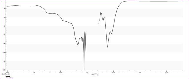
Radar RCS Graph
Summary
You created a scenario that used the surface of the WGS84 as the central body obstruction. You created a simple flight route of an aircraft and changed its RCS value to simulate a large, four-engined turboprop using a constant analytical RCS value. You created an airfield radar site and inserted a Sensor to create a servo system that was used to steer a radar antenna pattern inside its field of view in order to analyze various targets. You built a Radar using specifications typically found on air surveillance radars. You analyzed Pdet values for large, medium, small, and very small targets focusing on Pdet, SNR, and Pulse Integration. Finally, you used a notional aspect dependent RCS file that demonstrated both analytical and visual differences when compared to a constant RCS sphere.
On your own
Throughout the tutorial, hyperlinks were provided that pointed to in depth information of various tools and functions. Now is a good time to go back through this tutorial and view that information. Here are a few things you can do:
- Move the radar site to an area that is using a local analytical terrain file and constrain your objects to use terrain for analysis.
- Go on the Internet to find RCS values for other target types and analyze their Pdet values.
- Change settings in the Radar's properties and see their effects on your analysis.