Part 3:
STK Pro, STK Premium (Air), STK Premium (Space), or STK Enterprise
You can obtain the necessary licenses for this tutorial by contacting AGI Support at support@agi.com or 1-800-924-7244.
The results of the tutorial may vary depending on the user settings and data enabled (online operations, terrain server, dynamic Earth data, etc.). It is acceptable to have different results.
Capabilities covered
This lesson covers the following capabilities of the Ansys Systems Tool Kit® (STK®) digital mission engineering software:
- STK Pro
Problem statement
Engineers and operators often need to determine the times one object can "access" (or see) another object. In addition, they need to impose constraints on accesses between objects to define what constitutes a valid access. These constraints could include elevation angle, sunlight or umbra restrictions, gimbal speed, range, and more. Engineers also require the ability to create reports and graphs that summarize static data
Solution
With the STK software, you can determine accesses between objects and generate reports to summarize your data. Building on your fundamental understanding of the STK software, use two important tools in the STK application — the Access tool and the Report & Graph Manager — to solve this problem.
What you will learn
Upon completion of this tutorial, you will understand the following:
- How the Access tool functions by creating accesses between two or more objects
- How to save data externally by exporting reports
- How to update a report's units of measure
- How to generate prebuilt reports using quick reports
- How to use the Stored View tool
- How to find and use data providers with the Report & Graph Manager
- How to create custom reports for your scenario
- How to create 3D Graphics dynamic data displays
Video guidance
Watch the following video. Then follow the steps below, which incorporate the systems and missions you work on (sample inputs provided).
Creating a new scenario
First, you must create a new scenario, then build from there.
- Launch the STK application (
 ).
). - Click
 Create a Scenarioin the Welcome to STK dialog box.
 - Enter the following in the STK: New Scenario Wizard:
- Click when you are done.
- Click Save (
 ) once the scenario loads. A folder with the same name as your scenario is created for you in the location specified above.
 - Verify the scenario name and location and click .
| Option | Value |
|---|---|
| Name | AccessReportsGraphs |
| Location | Default |
| Start | Date: Default / Time: 18:00:00.000 UTCG |
| Stop | + 24 hr |
Save (![]() ) often during this lesson!
) often during this lesson!
Creating the satellite tracking station
A teleport facility, which is used to track satellites, is located in Castle Rock, Colorado.
Inserting a new Facility object
Insert Castle Rock Teleport into the scenario as a Facility object.
- In the Insert STK Objects tool (
 ), select Facility (
 ) in the Select An Object To Be Inserted list.
 - Select From Standard Object Database (
 ) in the Select a Method list.
 - Click .
- Enter Castle Rock in the Name field when the Search Standard Object Data dialog box opens.
- Click .
- Select the entry in the Results list whose Facility Name is Castle Rock Teleport and whose Network is INTELSAT.
- Click .
- Click to close the Search Standard Object Data dialog box.
Viewing the tracking station in 3D
View the Castle Rock Teleport in the 3D Graphics window.
- Bring the 3D Graphics window to the front.
- Right-click on Castle_Rock_Teleport () in the Object Browser.
- Select Zoom To in the shortcut menu.
- Use your mouse to get a good view of Castle_Rock_Teleport () and the surrounding terrain.
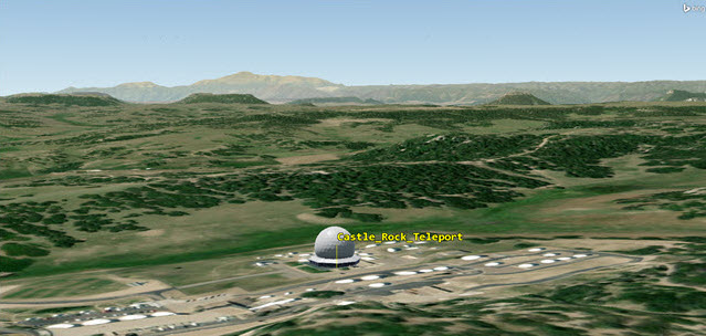
Castle Rock Teleport and Surrounding Terrain
Streaming terrain from a Terrain Server
- Right-click on ) in the Object Browser.
- Select Properties (
 ) in the shortcut menu.
 - Select the Basic - Terrain page when the Properties Browser opens.
- Clear the Use terrain server for analysis check box in the Terrain Server panel.
- Click to accept your changes and to close the Properties Browser.
- Bring the 3D Graphics window to the front.
Editing Castle Rock Teleport's properties
Castle_Rock_Teleport now appears to be floating above the terrain surface by several kilometers. The STK application is still referencing the Facility object's altitude based on the facility's altitude from the Standard Object Database.
- Open Castle_Rock_Teleport's () Properties ().
- Select the Basic - Position page when the Properties Browser opens.
- Select the Use terrain data check box in the Position panel.
- Click to accept your changes and to keep the Properties Browser open.
- Return to the 3D Graphics window.
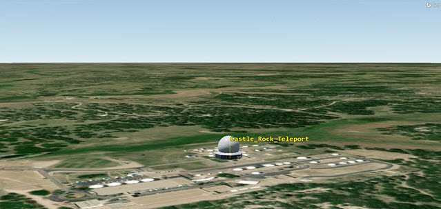
Castle Rock Teleport On Top of the WGS84 ellipsoid
The Castle_Rock_Teleport Facility object is now referencing the surface of the WGS84 ellipsoid.
Understanding access
The simplest definition of "access" is the ability of one object to see another object during a period of time. An
Understanding access constraints
The first condition for access is geometric line of sight, meaning the ability to draw a straight line between the positions of two objects. Additionally, there may also exist other conditions for access, called constraints.
- Return to Castle_Rock_Teleport's () Properties ().
- Select the Constraints - Active page.
- Click to close the Properties Browser without making any changes.
Note that the Line of Sight constraint is selected. The Line of Sight constraint computes whether the line of sight between two objects is obstructed by the ground, or, in this case, the WGS84 ellipsoid.
Attaching a Sensor object to Castle Rock Teleport
You can also restrict and visualize Castle_Rock_Teleport's field of view by using a Sensor object that models the properties of the antennas at the site.
- Insert a Sensor (
 ) object using the Insert Default () method.
 - Select Castle_Rock_Teleport () when the Select Object dialog box opens.
- Click .
- Right-click on Sensor1 () in the Object Browser.
- Select Rename in the shortcut menu.
- Rename Sensor1 () CR_FOV.
CR_FOV is an acronym for Castle Rock field of view.
Setting the half angle of the sensor
A
- Open CR_FOV's () Properties ().
- Select the Basic - Definition page.
- Enter 90 deg in the Cone Half Angle field.
- Click to accept your changes and to keep the Properties Browser open.
Pay attention to half angles. In this instance you are setting a half angle of 90 degrees. Therefore, your field of view is actually 180 degrees.
Setting the Sensor's constraints
- Select the Constraints - Active page.
- Click Add new constraints (
 ) in the Active Constraints toolbar.
 - Type Range in the Search field when the Select Constraints to Add dialog box opens.
- Select Range in the Constraint Name list.
- Click .
- Click to close the Select Constraints to Add dialog box.
- Select the Max check box in the Constraint Properties Range panel.
- Enter 1500 km in the Max field.
- Click to accept your changes and to close the Properties Browser.
Viewing the sensor's field of view in 3D
View the sensor's constrained field of view in the 3D Graphics window.
- Bring the 3D Graphics window to the front.
- Zoom To Castle_Rock_Teleport ().
- Zoom out enough to see CR_FOV's () field of view.
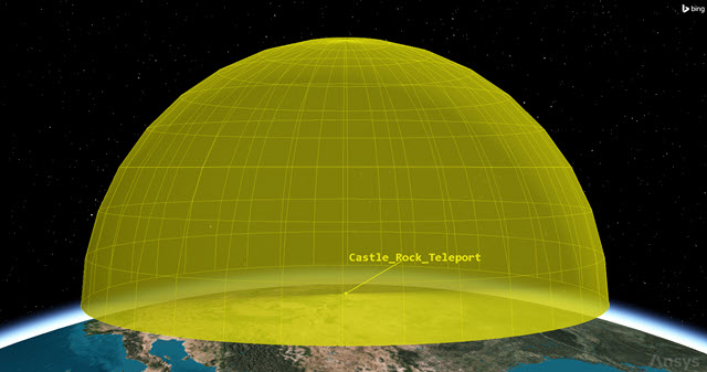
Castle rock Teleport's field of view
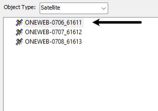
Inserting OneWeb satellites
Use the Standard Object Database to propagate five OneWeb satellites into your scenario.
Inserting satellites from the Standard Object Database
You'll use a select subset of satellites to calculate access from your sensor. Use the options available in the Standard Object Database to limit your search to those OneWeb satellites with an inclination between 87 and 90 degrees.
- Insert a Satellite (
 ) object using the From Standard Object Database () method.
 - Enter OneWeb in the Name or ID field when the Search Standard Object Data dialog box opens.
- Scroll down to Inclination.
- Select the Min check box.
- Enter 87 deg in the Min field.
- Select the Max check box.
- Enter 90 deg in the Max field.
- Click .
Selecting the most currently launched satellites
You will select the five most recently launched satellites.
- In the Results list, click on the Space Surveillance Catalog Number column header.
- You should see an upward-facing arrow.
- Click on the arrow so it points downward.
- Select the first five satellites whose Data Source is AGI's Standard Object Database.
- Click .
- Click to close the Search Standard Object Data dialog box after all five Satellite () objects have been propagated.

Up arrow
This should sort the list so that the newest satellites are now at the top.
If you don't have an Internet connection, pick the first five satellites, but make sure your local install is using the most recent Two Line Element (TLE) files that are available. For information on how to obtain the most current TLE files, refer to the
Using the Access tool
The
Computing access
You want to analyze if any OneWeb satellites pass through CR_FOV's field of view.
- Click Access... (
 ) in the STK Tools toolbar.
 - Click to the right of the Access for field when the Access tool opens.
- Select CR_FOV () in the Select Object dialog box.
- Click .
- Multi-select all the Satellite () objects in the Associated Objects list.
- Click

When the Access tool opens, the object currently selected in the Object Browser is selected as the primary object. This is denoted in the Access For field at the top of the tool.
"Access for" now shows Castle_Rock_Teleport-CR_FOV. This is the object from which you're looking.
You are computing access from CR_FOV to all the Satellite objects. You can see that once you compute the access, the Satellite objects' graphics have changed in the list. The names of the Satellite objects are now in bold and are marked with an asterisk. There is also a key (![]() ) icon with a green (
) icon with a green (![]() ) check mark, which represents a computed access. In the 2D Graphics window, there is a static highlight between the two objects. In the 3D Graphics window, a line connects the two objects when you animate the scenario and the objects have access each other.
) check mark, which represents a computed access. In the 2D Graphics window, there is a static highlight between the two objects. In the 3D Graphics window, a line connects the two objects when you animate the scenario and the objects have access each other.
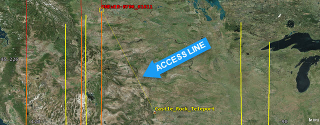
Viewing accesses in the 2D Graphics window
Prior to generating any reports or graphs, you can quickly view any accesses you might have been looking at the 2D Graphics window. The Graphics options available via the Access tool allow you to define the display of the access intervals in the 2D Graphics window.
- Bring the 2D Graphics window to the front.
- Click Zoom In (
 ) in the 2D Window Defaults toolbar.
 - Hold down your left mouse button, draw a box around and center your view on Castle_Rock_Teleport ().
- Use your mouse's scroll wheel to zoom out until you see the access lines in the vicinity of Castle_Rock_Teleport ().
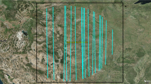
2D Graphics Access Lines
Your view will differ from the one shown here. The access lines don't tell you which satellite was seen, but shows you when satellites passed through the sensor's field of view and the sensor accessed them.
Viewing the access intervals in the Timeline View
The Timeline View can be used to visualize a variety of time intervals within your scenario.
- Look at the Timeline View.
- Return to the Access tool.
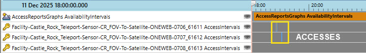
Timeline View with Access Intervals
Your view will differ from the one shown here. You can see multiple accesses and the times that actual access intervals occur. It's possible, depending on your analysis period, that some or all of your satellites will not have an access.
Generating an Access report
In the Access tool's Reports panel, you can generate an
- Ensure all the satellites are selected in the Associated Objects list.
- Click in the Reports panel.
- Scroll through the report to become familiar with the layout.
- Close the Access report once you are done.
- Leave the Access tool open.
If there is an access between the Sensor object and a Satellite object, the Access report tells you when, and for how long, the access takes place. If an access doesn't exist, the report will say No Access Found.
Generating an Access graph
In the Access tool's Graphs panel, you can generate an
- Return to the Access tool.
- Click in the Graphs panel.
- Locate the first access in the graph.
- Using your mouse, hold down the left mouse button and draw a box around the access.
- Place the cursor at the beginning of the access. A text box will appear with information about the access start time.
- When you are done, click Zoom Out (
 ) until you see the whole graph.
 - Close the Access graph when you are finished.
- Leave the Access tool open.
When you generate a graph, the zoom in function is automatically on.
This can be done multiple times until the graph is filled with the one access.
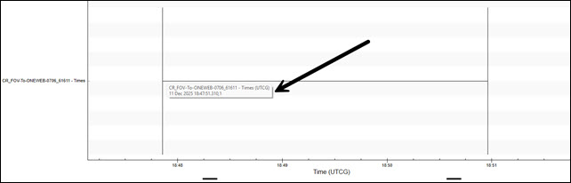
Graph with Access Start Time
Your view will be different than the one above.
Generating an Azimuth Elevation Range (AER) report
In the Reports and Graphs panels, you can generate an
- Return to the Access tool.
- Ensure all the satellites are selected in the Associated Objects list.
- Click in the Reports panel.
- Scroll through the report to become familiar with the layout.
- Close the AER report once you are done.
- Leave the Access tool open.
Since the access is taking place from an object on the ground, an azimuth of zero (0) degrees is True North. The elevation is based on the central body (the WGS84 ellipsoid). The range is calculated from the center point of the FROM object to the center point of the TO object. Remember, the Satellite objects must enter the Sensor object's field of view in order to be accessed.
Exporting reports and graphs
There are times when you create a report or graph and you want to save the original data because you are going to make property changes to one or all of the objects used in the report or graph. Maybe you need to save a report as a text file (.txt) in order to parse the data with a script. You might need to save the data as a spreadsheet. Are you creating a slide presentation? You can save your graphs as Bitmap files (.bmp), Joint Photographic Experts Group file (.jpg), and other image formats.
Creating Access reports
Create an Access report for the Satellite objects in your scenario so you can focus on the one Satellite object that has the longest total duration.
- Return to the Access tool.
- Click in the Reports panel.
- Review the report to find the satellite which has the longest total access duration.
- Close the Access report.
- Select the Satellite () object in the Associated Objects list which had the longest total duration in the Access report for all the satellites.
- Click in the Reports panel.
- Note the total number of accesses and the total duration.
This will create a combined report for all of the selected satellites.
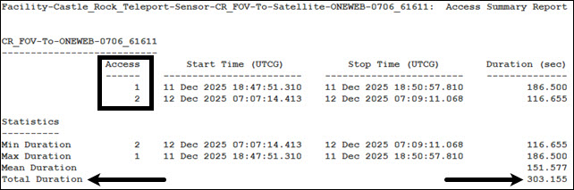
Number of Accesses and Total Duration
Your satellite and total duration values wont match what you see in this image.
This will create a report just for the one selected satellite.
Saving a report as a text document
Save your report as a text file.
- Click Save as text () in the reports toolbar.
- Ensure you are saving to your scenario folder (AccessReportsGraphs) when the Save Report dialog box opens.
- Enter Castle Rock to OneWeb in the File name field.
- Click .
Viewing the text document outside of the STK application
You can use the text editor of your choice (for example, Notepad or Notepad++) to open the report you just created. The data are outside of the STK application, so any further property changes to the objects won't be reflected in this report.
- Open Windows File Explorer.
- Browse to your scenario folder (for example, C:\Users\<username>\Documents\STK_ODTK 13\AccessReportsGraphs).
- Double-click on the text document named Castle Rock to OneWeb.txt to open the file.
- Close the text document once you are done.
- Close Windows File Explorer.
- Return to your Access report in the STK application.
As you can see, the text document is similar to the STK Access report format.
Saving an external .csv file
Clicking Save as .csv (![]() ) allows you to save the report which you can open using Excel.
) allows you to save the report which you can open using Excel.
Using other report options
If you right-click in the report and select the Export shortcut menu, you will get the following additional export format choices:
- To Excel: Exports data to Excel as a CSV or text file.
- To CSV Format: Exports data to Excel as a CSV file.
- Complete: Exports data to Excel as a CSV file. It includes summary information, such as minimum and maximum calculations.
- Setup: Sets export options for your report.
To understand all your options, see the Working with Reports help page.
Saving an external graph
To save a graph externally, you first generate the graph, then click Save as text (![]() ). You get the option of saving it in a number of formats, including bitmap (.bmp), metafile (.emf), JPEG (.jpg), Windows metafile (.wmf), and portable network graphics (.png).
). You get the option of saving it in a number of formats, including bitmap (.bmp), metafile (.emf), JPEG (.jpg), Windows metafile (.wmf), and portable network graphics (.png).
To understand all your options, see the Working with Graphs help page.
Extending CR_FOV's range
Extend the CR_FOV Sensor object's range to see how it affects your data.
- Open CR_FOV's () Properties ().
- Select the Constraints - Active page when the Properties Browser opens.
- Select Range in the Active Constraints list.
- Enter 2000 km in the Range panel's Max field.
- Click to accept your change and to close the Properties Browser.
Refreshing the Access report
Your Access report is showing the old data. Apply the new range constraint to the report.
- Return to your Access report.
- Click Refresh (F5) (
 ) in the Access report toolbar. You also have the option of selecting the F5 key to refresh a report.
 - Compare your new data to your old data.
- Do you have the same number of accesses?
- Are your durations longer?
Changing the report's units
![]() ) opens the Units dialog box that allows you to change the units of measure for the report. The Units dialog box will display all dimensions relevant to the report.
) opens the Units dialog box that allows you to change the units of measure for the report. The Units dialog box will display all dimensions relevant to the report.
- Click Report Units (
 ) in the report toolbar.
 - Select the Time Dimension in the Units Access dialog box.
- Select Minutes (min) in the New Unit Value list.
- Click .
- The Duration is now reported in minutes instead of seconds.
Using quick reports
A
Saving a new quick report
Save your Access report as a new quick report.
- Click Save as quick report (
 ) in the Access report toolbar.
 - Close the Access report.
- Close the Access tool.
Using the Quick Report Manager
The Quick Report Manager displays the entire list of quick reports that you have saved in your scenario. A quick report retains the customized object, time and unit settings of the displayed report or graph.
- Click Quick Report Manager... (
 ) in the Data Providers Toolbar.
 - Enter Sensor to OneWeb in the Name column when the Quick Report Manager opens.
- Select the Enter key.
- Clear the Show on Load check box if it's checked.
- Click .
- Close the Access report.
- Click to close the Quick Report Manager.
You can add any text to the Description field.
Show on Load will automatically open the report whenever you open the scenario.
This enables you to create the Access report without having to use the Access Tool.
Viewing the quick report
With your quick report created, open it from the Quick Report Manager using the drop-down menu.
- Open the Quick Report Manager () drop-down menu.
- Select Sensor to OneWeb (
 ).
). - Leave the Access report open.
Setting the Scenario Time from a report
Using the quick report (Access report), there are a couple of simple ways to set your animation time from the report. You will focus on the first access start time.
Using the shortcut menu
There are two ways you can set the animation time from your report; one is to use the shortcut menu.
- Right-click on the first access start time in the report.
- Select Start Time in the shortcut menu.
- Select Set Animation Time in the Start Time submenu.
- Look in the Animation Toolbar's Current Scenario Time field. It matches the start time of the first access.
- Click Reset (
 ) in the Animation Toolbar.
Copying the animation time from the report
Another way is to copy and paste a particular time from your report to the Current Scenario Time field.
- Return to the Access report.
- Highlight the first access start time.
- Right-click on the highlighted time.
- Select Copy (
 ) in the shortcut menu.
 - Click inside the Current Scenario Time field.
- Right-click on the highlighted time.
- Select Paste (
 ) in the shortcut menu.
 - Make sure the time is highlighted in the Current Scenario Time field.
- Select the Enter key.
- Close the Access report.
The Ctrl+C keyboard shortcut will also work.
The Ctrl+V keyboard shortcut will also work.
Your scenario's animation has jumped to the first instance that CR_FOV accesses your selected OneWeb satellite.
Using the Stored View tool
Use the Stored View tool to store the current view from your 3D Graphics window. When you store a view, that view includes all of the 3D Graphics window properties and the window position and direction settings. Therefore, it is important to make sure that you manipulate the view and set all properties exactly the way you want them before saving or modifying a view.
Setting up for a stored view
Configure your 3D Graphics window for the view you want to create.
- Bring the 3D Graphics window to the front.
- Zoom to the OneWeb satellite from the Access report.
- Adjust the view so that you can see the selected OneWeb satellite and Castle_Rock_Teleport ().
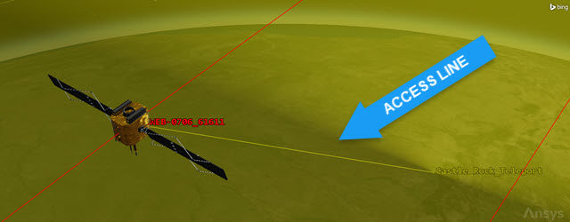
3D view Castle rock accesses a oneweb satellite
Your view will differ from the one shown here. The 3D Graphics window view shows the moment your selected OneWeb satellite enters CR_FOV's field of view. The line that appears between the OneWeb satellite and Castle Rock is an access line.
Viewing the access in the 2D Graphics window
You can view the access in the 2D Graphics window.
- Bring the 2D Graphics window to the front.
- Adjust your view so that you can see your selected OneWeb satellite and Castle_Rock_Teleport ().
2D view: Castle rock accesses a oneweb satellite
Your view will differ from the one shown here. The 2D Graphics window view shows the moment your selected OneWeb satellite enters CR_FOV's field of view. The line that appears between your selected OneWeb satellite and Castle Rock is an access line.
Creating a new stored view
Create a new stored view at the moment of first access between your selected OneWeb satellite and CR_FOV.
- Bring the 3D Graphics window back to the front.
- Make sure you have a good view of your selected OneWeb satellite, CR_FOV () and part of the sensor's field of view in the background.
- Click Stored Views (
 ) in the 3D Graphics toolbar.
 - Click in the Stored View 3D Graphics 1 - Earth dialog box.
- Change the View Name of view0 to Sat First Access.
- Click .
Selecting a stored view
With your stored view created, reset your animation time and view to see the change.
- Click Reset () in the Animation Toolbar.
- Click Home View (
 ) in the 3D Graphics toolbar.
 - Open the Stored Views () drop-down menu.
- Select Sat First Access.
The 3D Graphics window jumps back to the view and the time set in the view.
Using the Report & Graph Manager
You can generate
- Reports that summarize static data
- Reports that update during animation. These reports, called dynamic displays, enable you to view changes to selected elements over a period of time
- Graphs that summarize static data
- Graphs that update during animation. These graphs, called strip charts, enable you to view changes to selected elements over a period of time
Opening the Report & Graph Manager
Open the Report & Graph Manager and focus on data for a single satellite.
- Click Report & Graph Manager... (
 ) in the Data Providers toolbar.
 - Change the Object Type to Satellite in the upper-left corner of the Report & Graph Manager.
- Select the OneWeb satellite you have been studying in the Object List.
Multiple objects can be selected, but for this scenario, focus on your selected OneWeb satellite.
Object Type selection for a Report or Graph
Your view will differ from the one shown here.
Defining the Time Period for the Report or Graph
You can specify the period of time during which data is reported. You can view the available options in the Time Properties panel. For this analysis, you will keep the default settings.
Managing report and graph styles
You can manage the report and graph styles.
- Ensure (
 ) the Installed Styles (
 ) folder in the Styles list is expanded.
 - Take a close look at the two entries for Classical Orbit Elements located in the Installed Styles () folder.
- Notice the lock icons on each.
- Select the Classical Orbit Elements (
 ) report.
 - Click .
- Take a look at the report.
- Close the Classical Orbit Elements report when you are finished.
- Return to the Report & Graph Manager.
- Look at the very top of the Styles field.
One is a graph style (![]() ) and one a report style (
) and one a report style (![]() ).
).
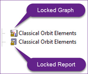
Locked Reports and Graphs
The reports and graphs located in the Styles list are read only and cannot be customized. However, they can be duplicated, and those duplicates can be customized.
The Classical Orbit Elements (![]() ) report is now available in the My Favorites (
) report is now available in the My Favorites (![]() ) folder.
) folder.
Understanding data providers, groups and elements
The content of any report or graph is generated from the selected data providers for the report or graph style.
Understanding data providers by object
View the data providers used for the Classical Orbit Elements report.
- Right-click on the Classical Orbit Elements () report in the Installed Styles () folder.
- Select Duplicate (
 ) in the shortcut menu.
 - Select the Content page when the Properties Browser opens.
- Look at the Report Contents list.
- Time
- Data Provider: Classical Elements
- Data Provider Group: J2000
- Data Provider Elements: Time (UTCG), Semi-major Axis (km), Eccentricity, etc.
- In the Report Contents list, select Classical Elements-J2000-Semi-major Axis.
- Look in the Data Providers list.
The left side shows all the data providers for the object type (in this case, a Satellite (![]() ) object) and on the right side are the Report Contents.
) object) and on the right side are the Report Contents.
The report is broken out into the following data providers, groups and elements:
You can see the hierarchy of Data Provider - Data Provider Group - Data Provider Element: in this case, Classical Elements (![]() ) - J2000 (
) - J2000 (![]() ) - Semi-major Axis (
) - Semi-major Axis (![]() ).
).
Customizing reports
You can customize the properties of a static or dynamic report.
Customizing the units of measure
Change units of measure for a report style or a displayed report.
- Return to the Report Contents list.
- Select Classical Elements-J2000-Semi-major Axis.
- Below Report Contents, click .
- Clear the Use Defaults check box in the Units dialog box.
- Select Meters (m) in the New Unit Value list.
- Click to close the Units dialog box.
The current distance unit is being reported in kilometers (km).
Your custom report will use meters instead of kilometers for the semi-major axis.
Removing the default data provider elements
Before adding any new data provider elements, remove some existing ones.
- In the Report Contents list, select the following:
- Classical Elements-J2000-Arg of Perigee
- Classical Elements-J2000-True Anomaly
- Classical Elements-J2000-Mean Anomaly
- Click .
Customizing the report's contents
As previously stated, you will replace argument of perigee, true anomaly and mean anomaly data provider elements with J2000 x, y, and z
- Remove the asterisk (*) at the top of the Data Providers list, in the Filter field.
- Enter Cartesian in the Filter field.
- Click .
- Expand () the Cartesian Position () data provider.
- Expand () the J2000 () data provider group.
- Move (
 ) the x, y, and z data providers (
 ) to the Report Contents list.
 - If desired, use the up (
 ) and down (
 ) arrows to place elements where desired.
 - Click to accept your changes and to close the Properties Browser.
This narrows down your choices to only those data providers containing Cartesian data providers, groups or elements.
Generating a custom report
With your new report style saved, generate your custom report.
- Expand () the My Styles () folder in the Styles list.
- Right-click on Classical Orbit Elements ().
- Select Rename in the shortcut menu.
- Rename Classical Orbit Elements () My Classical Orbit Elements.
- Click
- Close the report when you are finished.
The custom report is showing the semi-major axis in meters and the J2000 X Y Z Cartesian Position elements. The report is in 60 second increments which can be changed in the Time Properties field if desired or selecting .
Creating a display of dynamic data
You can generate reports that update during animation. These reports, called dynamic displays or strip charts, enable you to view changes to selected elements over a period of time.
Generating a new dynamic display
- Ensure the My Classical Orbit Elements () report is selected.
- Select the Dynamic Display/Strip Chart option in the Generate As field in the Styles panel.
- Click .
- Click Reset () in the Animation toolbar.
- Click X Real-time Animation Mode (
 ).
). - Click Start (
 ) to animate the report.
 - Click Reset () when finished.
- Close all open reports and the Report & Graph Manager.
The dynamic display updates as the scenario animates.
Creating a new dynamic 3D Graphics data display
The 3D Graphics Data Display properties allow you to display dynamic data for the specified object in the 3D Graphics window. This feature is useful when presenting information that requires both visual and textual data. If you record a movie of your scenario, the data will appear in the movie.
- Open your selected OneWeb satellite's Properties ().
- Select the 3D Graphics - Data Display page.
- Click .
- Select My Classical Orbit Elements in the Styles list when the Add a Data Display dialog box.
- Click to close the Add a Data Display dialog box.
- Click to accept your changes and to close the Properties Browser.
Settings in the Position panel automatically places the data in the top left portion of the 3D Graphics window. You can add more data to the window and then change the position. Note other selections for appearance and background.
Viewing the dynamic data display in action
View your dynamic data display in the 3D Graphics window.
- Bring the 3D Graphics window to the front.
- Open the Stored Views () drop-down menu.
- Select Sat First Access.
- Click Start () in the Animation toolbar to animate the scenario. Data updates dynamically in the 3D Graphics window.
- Click Reset () when finished.
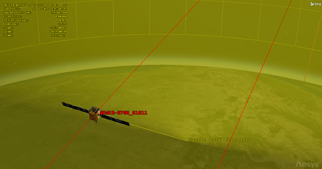
3D Graphics Window Dynamic Data
Your view will differ from the above image. The stored view now shows the moment your selected OneWeb satellite enters CR_FOV's field of view and important data pertaining to the satellite is displayed in the 3D Graphics window.
Summary
![]() ) object. Next, you propagated multiple OneWeb satellites.
) object. Next, you propagated multiple OneWeb satellites.
Continue to Lesson Four: Movies and Visual Data Files.
On your own
Throughout the tutorial, hyperlinks were provided that pointed to in depth information of various subjects. Now's a good time to go back through this tutorial and view that information. Try creating new views or custom reports. Place a Sensor object on a Satellite object, add cities from the city database, and create accesses from the Satellite object to the ground sites. Explore and have fun!