Part 7:
STK Pro, STK Premium (Air), STK Premium (Space), or STK Enterprise
You can obtain the necessary licenses for this tutorial by contacting AGI Support at support@agi.com or 1-800-924-7244.
This tutorial requires STK 12.9 or newer to complete in its entirety. If you have an earlier version of STK, you can view a legacy version of this lesson.
The results of the tutorial may vary depending on the user settings and data enabled (online operations, terrain server, dynamic Earth data, etc.). It is acceptable to have different results.
Capabilities covered
This lesson covers the following capability of the Ansys Systems Tool Kit® (STK®) digital mission engineering software:
- STK Pro
- Analysis Workbench
Problem statement
Engineers and technicians require additional capabilities when using the STK application to create custom functions and calculations relative to times, positions, and reference frames. You work at a ground station that is tracking a geosynchronous satellite. The ground station's sensor must be monitored for its safety when its boresight is within 30 degrees of the Sun so that it won't be damaged. You require data that informs you when the sensor's boresight is within that 30-degree range and when it's outside of that same 30-degree range.
Solution
Use a combination of STK Pro and the STK software's Analysis Workbench capability to create vectors, custom angles, calculations, time components and temporal constraints to determine when the sensor can safely track the satellite.
What you will learn
Upon completion of this tutorial, you will understand the following:
- How to access and use the Analysis Workbench
- How to use the Vector Geometry tool
- How to use the Time tool
- How to use the Calculation tool
Video guidance
Watch the following video. Then follow the steps below, which incorporate the systems and missions you work on (sample inputs provided).
Creating a new scenario
First, you must create a new STK scenario and then build from there.
- Launch the STK application (
 ).
). - Click
 Create a Scenario in the Welcome to STK dialog box.
 - Enter the following in the STK: New Scenario Wizard:
- Click when you finish.
- Click Save (
 ) when the scenario loads.
 - Verify the scenario name and location in the Save As dialog box.
- Click .
| Option | Value |
|---|---|
| Name | STK_AnalysisWorkbench |
| Location | Default |
| Start | Today |
| Stop | + 5 days |
By using Today as the Start time, every time you open the scenario, it will automatically adjust to the current date, using midnight local time and its equivalent Universal Time Coordinated Gregorian (UTCG) date unless your chose a different time unit for your scenario. This is useful when you want to track Satellite objects that you have inserted into the scenario.
The STK software creates a folder with the same name as your scenario for you.
Save (![]() ) often during this tutorial!
) often during this tutorial!
Disabling streaming terrain
Streaming terrain is not required for this analysis. Disable the Terrain Server.
- Right-click on STK_AnalysisWorkbench () in the Object Browser.
- Select Properties (
 ) in the shortcut menu.
 - Select the Basic - Terrain page when the Properties Browser opens.
- Clear the Use terrain server for analysis check box in the Terrain Server panel.
- Click to confirm your change and to close the Properties Browser.
Modeling the ground station
The satellite tracking ground station is located at the Kaena Point Space Force Station on Oahu, Hawaii. Model the station with a Facility object. A Facility object models a ground station or other facility on the surface of the central body.
Inserting the Facility object
Insert a new Facility object from your locally installed
- Bring the Insert STK Objects tool (
 ) to the front.
 - Select Facility (
 ) in the Select An Object To Be Inserted list.
 - Select From Standard Object Database (
 ) in the Select A Method list.
 - Click .
- If online operations are enabled, clear the Data Sources: Online check box when the Search Standard Object Data dialog box opens.
- Enter Kaena In the Name field located under Data Sources.
- Click .
- Select Kaena Point Radar STDN KPTQ in the Results list.
- Click .
- Click to close the Search Standard Object Data dialog box.
Adding the facility's lighting intervals to the Timeline View
Lighting intervals are the periods of full lighting (sunlight), partial lighting (penumbra) and zero lighting (umbra). The
- Click Add Time Components (
 ) on the Timeline View toolbar.
 - Select Kaena_Point_Radar_STDN_KPTQ () in the Objects list when the Select Timeline Component dialog box opens.
- Select LightingIntervals (
 ) in the Components for: Kaena_Point_Radar_STDN_KPTQ list.
 - Click to confirm your selection and to close the Select Timeline Component dialog box.
Lighting intervals for STK objects are computed automatically by the STK software and are made available for use by default. You can also use the Analysis Workbench capability's Time tool to create custom intervals.
Viewing Kaena_Point_Radar_STDN_KPTQ in the 3D Graphics window
Use the Timeline View to view Kaena_Point_Radar_STDN_KPTQ in sunlight.
- Right-click on Kaena_Point_Radar_STDN_KPTQ () in the Object Browser.
- Select Zoom To in the shortcut menu.
- Move the Timeline View's gray pointer (
 ) to a Sunlight interval so you can better see the facility in the 3D Graphics window.
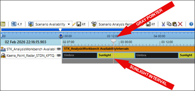
Gray pointer and sunlight interval
Note that the facility seems to be floating above the terrain. When you bring a Facility object into your STK scenario using the From Standard Object Database method, the Facility object is automatically placed at the actual altitude of the terrain at that location.
Adjusting the altitude of Kaena_Point_Radar_STDN_KPTQ
Since you're using the WGS84 ellipsoid's surface in your analysis, Kaena_Point_Radar_STDN_KPTQ's altitude needs to be modified. Adjust it so that it sits on the surface of the WGS84 ellipsoid by updating the facility's
- Open Kaena_Point_Radar_STDN_KPTQ's () Properties ().
- Select the Basic - Position page when the Properties Browser opens.
- Select the Use terrain data check box in the Position panel.
- Click to confirm your selection and to close the Properties Browser.
Kaena_Point_Radar_STDN_KPTQ is now sitting on the surface of the WGS84 ellipsoid.
Inserting a Satellite object
Insert a Satellite object, which will be tracked by Kaena_Point_Radar_STDN_KPTQ. In this scenario you will build a nominal Satellite object using the Orbit Wizard.
Inserting a satellite from the Orbit Wizard
The
- Bring the Insert STK Objects tool () to the front.
- Insert a Satellite (
 ) object using the Orbit Wizard (
 ) method.
 - Set the following options when the Orbit Wizard opens:
- Click to propagate GEO_Sat () and to close the Orbit Wizard.
| Option | Value |
|---|---|
| Type | Geosynchronous |
| Satellite Name | GEO_Sat |
| Subsatellite Point | -150 deg |
Updating GEO_Sat's orbit epoch.
It's important to note that should you open this scenario in the future using GEO_Sat, you will need to match the orbit epoch to the day you open the scenario. You can change it by updating GEO_Sat's
- Open GEO_Sat's () Properties ().
- Select the Basic - Orbit page when the Properties Browser opens.
- Locate the Orbit Epoch field.
- Open the drop-down menu (
 ) next to Orbit Epoch.
 - Select Set to Today in the drop-down menu.
- Click to confirm your selection and to close the Properties Browser.
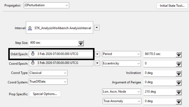
orbit epoch
The time at which the established orbital elements are true will now update with your scenario time, should you choose to reopen it.
Computing access
Calculate the times Kaena_Point_Radar_STDN_KPTQ can
- Right-click on Kaena_Point_Radar_STDN_KPTQ () in the Object Browser.
- Select Access... (
 ) in the shortcut menu.
 - Select GEO_Sat () Associated Objects list when the Access tool opens.
- Click
 .
. - Look at the Timeline View.
- Click to close the Access tool.
There is one continuous access interval between Kaena_Point_Radar_STDN_KPTQ and GEO_Sat.
Displaying installed components from the Analysis Workbench
The Analysis Workbench capability comprises four application-wide tools (the Vector Geometry tool, the Time tool, the Calculation tool, and the Spatial Analysis tool) that you can use to create custom components and insert them into your scenarios. They are designed to streamline, organize, and extend the fundamental computational capabilities of the STK software. You can use these tools to create components that suit your needs.
The Analysis Workbench capability also contributes an extensive list of predefined components to the STK application that you can use immediately. Any of the components created by you or already installed can be used to report, graph, create data files, and visualize 2D and 3D time-dynamic data. You can design your computational tasks by combining different types of components from the Analysis Workbench.
Among the available components are the Facility object's Lighting intervals, which you added earlier, and its Sun Vector. Visualize this vector to aid in the design of your computation.
Displaying Kaena_Point_Radar_STDN_KPTQ's Sun vector
Vectors define directions in 3D space as well as magnitude. The Sun Vector is the apparent position of the Sun with respect to the object as a function of time. In this scenario, the Sun vector is anchored to tracking station's center point and targets the Sun. Enable the display of the vector by updating Kaena_Point_Radar_STDN_KPTQ's
- Open Kaena_Point_Radar_STDN_KPTQ's () Properties ().
- Select the 3D Graphics - Vector page when the Properties Browser opens.
- Select the Vectors tab.
- Select the Sun Vector Show check box.
- Click to confirm your selection and keep the Properties Browser open.
Viewing the Sun Vector
View the Sun Vector in the 3D Graphics window.
- Bring the 3D Graphics window to the front.
- Zoom to Kaena_Point_Radar_STDN_KPTQ ().
- Zoom out far enough so that you can see the Sun vector.
When you animate the scenario, the Sun vector will always follow the Sun.
Adding a To Vector
A To Vector is a displacement vector between origin and destination object points. To Vectors are automatically generated by STK for all objects in your scenario. The vectors are stored in a separate folder labeled "To Vectors," unless a vector with the same name already exists (Earth or Sun). In scenarios with many objects, the To Vectors folder can be very large for each object. Enable the display of the facility's To Vector to GEO_Sat.
- Return to Kaena_Point_Radar_STDN_KPTQ's () 3D Graphics - Vector Properties ().
- Click .
- Select Kaena_Point_Radar_STDN_KPTQ () in the Objects list when the Add Components dialog box opens.
- Expand (
 ) the To Vectors (
 ) folder in the Components for: Kaena_Point_Radar_STDN_KPTQ list.
 - Select GEO_Sat (
 ).
). - Click to confirm your selection and to close the Add Components dialog box.
The
Notice that GEO_Sat Vector is now added to the Vectors list, and the Show check box is already selected.
Showing the vector's magnitude
If Show Magnitude is selected, the magnitude (distance) value is displayed on the selected vector. This is only available for vectors. Turn on the magnitude for GEO_Sat's To Vector.
- Ensure GEO_Sat Vector is highlighted in the Vectors list.
- Select the Show Magnitude check box below the Vectors list.
- Click to confirm your selection and to keep the Properties Browser open.
- Bring the 3D Graphics window to the front.
Notice that the GEO_Sat To Vector now shows how far away GEO_Sat is located from Kaena_Point_Radar_STDN_KPTQ. When you animate the scenario, the GEO_Sat To vector will always point to GEO_Sat.
Using the Vector Geometry tool
The Analysis Workbench capability's Vector Geometry tool creates geometry components with time-varying placement or orientation in 3D space, including Vectors (![]() ), Axes (
), Axes (![]() ), Points (
), Points (![]() ), Systems (
), Systems (![]() ), Angles (
), Angles (![]() ), and Planes (
), and Planes (![]() ). Use the Vector Geometry tool to create an angle between Sun vector and the GEO_Sat To vector. For the purposes of this scenario, whenever the angle is 30 degrees or less, the satellite tracking system needs to be monitored.
). Use the Vector Geometry tool to create an angle between Sun vector and the GEO_Sat To vector. For the purposes of this scenario, whenever the angle is 30 degrees or less, the satellite tracking system needs to be monitored.
Opening the Analysis Workbench
Access the Vector Geometry tool by opening the Analysis Workbench.
- Right-click on Kaena_Point_Radar_STDN_KPTQ () in the Object Browser.
- Select Analysis Workbench... (
 ) in the shortcut menu.
 - Select the Vector Geometry tab when the Analysis Workbench opens.
Creating a Between Vectors angle
Create an angle between the Sun Vector and the GEO_Sat Vector using a Between Vectors angle type. A Between Vectors Angle type defines an angle between two vectors.
- Select Kaena_Point_Radar_STDN_KPTQ () in the Objects list on the left side of the browser.
- Click Create new Angle (
 ) in the Vector Geometry toolbar.
 - Ensure the Type is set to Between Vectors when the Add Geometry Component dialog box opens.
- Enter Tracking Angle in the Name field.
Selecting the From Vector
Select GEO_Sat's To Vector as the angle's From Vector. The custom angle, Tracking Angle, will be measured starting from GEO_Sat's To Vector.
- Click the From Vector ellipsis (
 ).
). - Select Kaena_Point_Radar_STDN_KPTQ () in the Objects list when the Select Reference Vector dialog box opens.
- Expand () the To Vectors () folder in the Vectors for: Kaena_Point_Radar_STDN_KPTQ list.
- Select GEO_Sat (
 ).
). - Click to confirm your selection and to close the Select Reference Vector dialog box.
Selecting the To Vector
Use the Sun Vector as the To Vector.
- Notice that Kaena_Point_Radar_STDN_KPTQ Sun is already selected for the To Vector.
- Click to confirm your changes and to close the Add Geometry Component dialog box.
- Keep the Analysis Workbench () open.
Displaying the tracking angle
Custom angles can be viewed in the 3D Graphics window. Add the custom tracking angle to Kaena_Point_Radar_STDN_KPTQ's 3D Graphics - Vector Properties page.
- Return to Kaena_Point_Radar_STDN_KPTQ's () 3D Graphics - Vector Properties ().
- Select the Angles tab.
- Click .
- Select Kaena_Point_Radar_STDN_KPTQ () in the Objects list when the Add Components dialog box opens.
- Select TrackingAngle (), located in the My Components () folder in the Components for: Kaena_Point_Radar_STDN_KPTQ list.
- Click to confirm you selection and to close the Add Components dialog box.
- Click to confirm your changes and to close the Properties Browser.
Viewing the tracking angle
View your custom tracking angle in the 3D Graphics window.
- Bring the 3D Graphics window to the front.
- Adjust your view so that you can see the Sun Vector, the To Vector and the Tracking Angle.
- Move the Timeline View's gray pointer () to animate the scenario.
![]()
Vectors and Angle View
Notice that as the scenario animates, the angle increases and decreases, updating dynamically.
Using the Calculation tool
Use the Calculation tool to determine when the tracking angle is 30 degrees or less. The Calculation tool defines components that produce time-varying computational results that can be reported, graphed, transformed, and analyzed further.![]() ), Conditions (
), Conditions (![]() ), and Parameter Sets (
), and Parameter Sets (![]() ).
).
Opening the Calculation tool
Open the Calculation tool from the Analysis Workbench.
- Return to Analysis Workbench.
- Select the Calculation tab to open the Calculation tool.
Defining a Scalar calculation
You will create a Scalar calculation to return the tracking angle values. A Scalar defines components that produce scalar time-varying calculations. Scalar calculation components also have the ability to return minimum, maximum, mean, and standard deviation values.
- Select Kaena_Point_Radar_STDN_KPTQ () in the Objects list.
- Click Create new Scalar Calculation (
 ) in the Calculation toolbar.
 - Ensure the Type is set to Angle when the Add Calculation Component dialog box opens.
- Enter Scalar Tracking Angle in the Name field.
- Click the Input Angle ellipsis ().
- Select Kaena_Point_Radar_STDN_KPTQ () in the Objects list when the Select Reference Angle dialog box opens.
- Select TrackingAngle (
 ), located in the My Components () folder in the Angles for: Kaena_Point_Radar_STDN_KPTQ list.
 - Click to confirm your selection and to close the Select Reference Vector dialog box.
- Click to confirm your changes and to close the Add Calculation Component dialog box.
The default scalar calculation type is Angle. The Angle type is an angular displacement specified by an Angle component from the Vector Geometry tool.
Defining a Condition
A condition defines a scalar calculation that is considered to be satisfied when it is positive and not satisfied when it is negative. Create a Scalar Bounds Condition to report when the tracking angle is 30 degrees or less. Scalar Bounds define a condition by combining a specified Scalar component with scalar bounds.
- Return to the Calculation tool.
- Select Kaena_Point_Radar_STDN_KPTQ () in the Objects list.
- Click Create new Condition (
 ) in the Calculation toolbar.
 - Ensure the Type is set to Scalar Bounds when the Add Calculation Component dialog box opens.
- Enter Below 30 Degrees in the Name field.
The default Calculation type is Scalar Bounds.
Selecting the Reference Scalar Calculation
Select the tracking angle scalar component you created earlier as the Reference Scalar Calculation.
- Click the Scalar ellipsis ().
- Select Kaena_Point_Radar_STDN_KPTQ () in the Objects list when the Select Reference Scalar Calculation dialog box opens.
- Select Scalar_Tracking_Angle (
 ), located in the My Components () folder in the Scalar Calculations for: Kaena_Point_Radar_STDN_KPTQ list.
 - Click to confirm your selection and to close the Select Reference Scalar Calculation dialog box.
Defining the Scalar Bounds' operation
Define the calculation condition of the Scalar Bounds to be 30 degrees or less by choosing an associated operation.
- Open the Operation drop-down list.
- Select Below Maximum.
- Enter 30 deg in the Maximum field.
- Click to confirm your changes and to close the Add Calculation Component dialog box.
When the values are at 30 degrees or below, the calculation will be satisfied.
Creating a report
You can create reports and graphs directly inside the Calculation tool. Create an
- Select Kaena_Point_Radar_STDN_KPTQ () in the Objects list.
- Expand () Below_30_Degrees (), located in the My Components () folder in the Components for: Kaena_Point_Radar_STDN_KPTQ list.
- Right-click on SatisfactionIntervals ().
- Select Report... in the shortcut menu.
- Close (
 ) the report.
 - Keep the Analysis Workbench open.
The report shows when the tracking angle is 30 degrees or less during the entire scenario interval.
Viewing the access intervals in the Timeline View
Use the Timeline View to visualize the times Kaena_Point_Radar_STDN_KPTQ has access to GEO_Sat and the times the tracking angle is less than 30 degrees.
- Click Add Time Components () in the Timeline View toolbar.
- Select Kaena_Point_Radar_STDN_KPTQ () in the Objects list when the Select Timeline Component dialog box opens.
- Expand () Below_30_Degrees (
 ), located in the My Components () folder in the Components for: Kaena_Point_Radar_STDN_KPTQ list.
 - Select SatisfactionIntervals (
 ).
). - Click to confirm your selection and to close the Select Timeline Component dialog box.
- Look in the Timeline View to view the intervals when the tracking angle at 30 degrees or below.
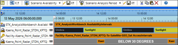
Below 30 Degree Satisfaction Intervals
Using the Time tool
Time is fundamental to most computations in STK and is used in reporting and graphing as well as in static and dynamic visualizations. Use the Time tool to create components that deal with time-related quantities.![]() ), Intervals (
), Intervals (![]() ), Interval Lists (
), Interval Lists (![]() ), Collections of Interval Lists (
), Collections of Interval Lists (![]() ), and Time Arrays (
), and Time Arrays (![]() ).
).
Opening the Time tool
Open the Time tool from the Analysis Workbench.
- Return to the Analysis Workbench.
- Select the Time tab.
Creating an Interval List
An Interval List Time component type defines components that produce an ordered list of time intervals. Create an Interval List to show when Kaena_Point_Radar_STDN_KPTQ has access to GEO_Sat while the tracking angle is above 30 degrees by merging the access intervals with the Below_30_Degrees satisfaction intervals. Subtract the Below_30_Degrees satisfaction intervals from the access intervals to define optimal tracking opportunities.
- Select Kaena_Point_Radar_STDN_KPTQ () in the Objects list.
- Click Create new Interval List (
 ) in the Time toolbar.
 - Click Type when the Add Time Component dialog box opens.
- Select Merged () in the Select Component Type list when the Select Component Type dialog box opens.
- Click to confirm your selection and to close the Select Component Type dialog box.
- Enter Optimal Tracking Times in the Name field.
A Merged Interval list contains intervals merged from multiple Interval or Interval List time components.
Defining the merging operation
Define the merge operation as Minus. The Minus operation is available when there are only two time components in the merge list. This will subtract the below 30-degree satisfaction intervals from the accesses to define optimal tracking opportunities.
- Open the Operation drop-down list.
- Select MINUS.
Removing the default time components
Remove the default time components.
- Select both Time Components in the Time Components list.
- Click .
Defining the Time Components
In this instance, there are two time components you need for your merged interval list: the accesses between the Kaena_Point_Radar_STDN_KPTQ and GEO_Sat and the Below_30_Degrees satisfaction intervals.
- Click .
- Select Facility-Kaena_Point_Radar_STDN_KPTQ-To-Satellite-GEO_Sat (
 ) in the Objects list when the Select Time Intervals dialog box opens.
 - Select AccessIntervals (), located in the Installed Components () folder in the Components for: Facility-Kaena_Point_Radar_STDN_KPTQ-To-Satellite-GEO_Sat list.
- Click to confirm your selection and to close the Select Time Intervals dialog box.
- Click .
- Select Kaena_Point_Radar_STDN_KPTQ () in the Objects list when the Select Time Intervals dialog box opens.
- Expand () Below_30_Degrees (), located in the My Components () folder in the Components for: Kaena_Point_Radar_STDN_KPTQ list.
- Select SatisfactionIntervals ().
- Click to confirm your selection and to close the Select Time Intervals dialog box.
- Click to confirm your changes and close the Add Time Component dialog box.
Viewing the Optimal Tracking Times Interval List in the Timeline View
You now have all the components for your analysis completed. View them in the Timeline View.
- Click Add Time Components () in the Timeline View toolbar.
- Select Kaena_Point_Radar_STDN_KPTQ () in the Objects list when the Select Timeline Component dialog box opens.
- Select Optimal_Tracking_Times (), located in the My Components () folder in the Components for: Kaena_Point_Radar_STDN_KPTQ list.
- Click to confirm your selection and to close the Select Timeline Component dialog box.
- Look at the Timeline View to see the all the time components.
- Return to the Analysis Workbench.
- Click to close the Analysis Workbench.
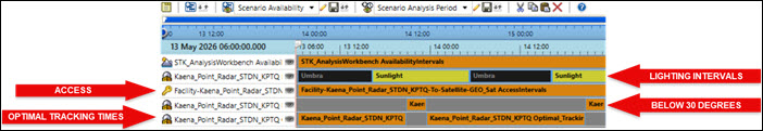
scenario time components
Modeling a sensor outage using components from the Analysis Workbench
You can use the custom components your created using the Analysis Workbench with other objects in the scenario for a variety of applications. Use your optimal tracking times Interval List to model a potential outage on a Sensor object attached to when the tracking angle goes below 30 degrees.
Attaching a Sensor object to Kaena_Point_Radar_STDN_KPTQ
Attach a
- Bring the Insert STK Objects tool () to the front.
- Insert a Sensor (
 ) object using the Define Properties () method.
 - Select Kaena_Point_Radar_STDN_KPTQ () when the Select Object dialog box opens.
- Click to confirm your selection and to close the Select Object dialog box.
Modeling a limited field of view
Set a limited field of view for the Sensor object to provide situational awareness. The
- Select the Basic - Definition page when the Properties Browser opens.
- Keep the default Simple Conic Sensor Type.
- Enter 5 deg in the Cone Half Angle field.
- Click to confirm your change and to keep the Properties Browser open.
A Simple Conic sensor type is defined by a specified cone half angle.
Targeting GEO_Sat
Use the Targeted pointing type to point the Sensor object at GEO_Sat.
- Select the Basic - Pointing page.
- Open the Pointing Type drop-down list.
- Select Targeted.
- Select GEO_Sat () in the Available Targets list.
- Move (
 ) GEO_Sat () to the Assigned Objects list.
 - Click to confirm your changes and to close the Properties Browser.
- Rename Sensor1 () Tracking_Sensor.
Computing access
Compute an access between the Tracking_Sensor and GEO_Sat.
- Right-click on Tracking_Sensor () in the Object Browser.
- Select Access... () in the shortcut menu.
- Select GEO_Sat () in the Associated Objects list when the Access tool opens.
- Click .
Generating an Access report
You can generate several types of reports and graphs that enable you to view specific types of access data directly from the Access tool. Generate an
- Click in the Reports panel.
- Return to the Access tool.
- Click to close the Access tool.
- Keep the Access report open.
Notice that there is one continuous access between Tracking_Sensor and GEO_Sat.
Adding a Temporal constraint
You want to know when Tracking_Sensor accesses GEO_Sat, but you want to remove access times from your report when Tracking_Sensor's boresight is within 30 degrees of the Sun. You can do this by adding a Temporal constraint to Tracking_Sensor using the custom components created in your scenario. Temporal constraints enable you to impose time-based constraints on an object.
- Open Tracking_Sensor's () Properties ().
- Select the Constraints - Active page when the Properties Browser opens.
- Click Add new constraints (
 ) in the Active Constraints toolbar.
 - Clear the All Categories check box in the Filter by Category list when the Select Constraints to Add dialog box opens.
- Select the Temporal check box.
- Select Intervals in the Constraint Name list.
- Click .
- Click to close the Select Constraints to Add dialog box.
Setting the Constraint Properties
Set the constraint to use the merged interval list you created earlier.
- Open the Source drop-down list in the Constraint Properties section.
- Choose Select time component.
- Click .
- Select Kaena_Point_Radar_STDN_KPTQ () in the Objects list when the Select Interval, Interval List or Interval Collection dialog box opens.
- Select Optimal_Tracking_Times (
 ), located in the My Components () folder in the Components for: Kaena_Point_Radar_STDN_KPTQ list.
 - Click to confirm your selection and to close the Select Interval, Interval List or Interval Collection dialog box.
- Notice that the Exclude Time Intervals check box is cleared.
- Click to confirm your changes and to close the Properties Browser.
The Access tool will only report accesses during the optimal tracking times. If you select the Exclude Time Intervals check box, then the Access report will show when the tracking angle is below 30 degrees.
Refreshing the Access report
The current Access report has one long access period for five days. Refresh the report so that it shows only those times that the tracking angle is above 30 degrees. These will be your optimal tracking times.
- Return to the Access report.
- Click Refresh (F5) (
 ) in the Access report toolbar.
 - Close the Access report.
You should only see those time that the tracking angle is above 30 degrees. If you look at the Timeline View, you'll see that the access between Tracking_Sensor and GEO_Sat matches the Optimal Tracking Times time component.
Viewing Tracking_Sensor in the 3D Graphics window
You can watch Tracking_Sensor turn on and off in the 3D Graphics window using the Timeline View.
- Bring the 3D Graphics window to the front.
- Zoom to Kaena_Point_Radar_STDN_KPTQ ().
- Use your mouse to zoom out far enough so that you can see Tracking_Sensor ().
- Move the Timeline View's gray pointer () over a couple of days while watching Tracking_Sensor () in the 3D Graphics window.
Tracking_Sensor will turn on during optimal tracking times and turn off during periods when the tracking angle is below 30 degrees.
Saving your work
Clean up and close out your scenario.
- Close any open tools and the Properties Browser.
- Save () your work.
Summary
This tutorial focused on three tools that are available in the Analysis Workbench: the Vector Geometry tool, the Time tool, and the Calculation tool. Using STK objects, you modeled a ground station tracking a geostationary satellite. After creating an access between the satellite and the tracking station, you displayed several available installed components from the Analysis Workbench in the 3D Graphics window. You used the Vector Geometry tool to create a custom angle between the vectors and the Calculation tool to create a scalar using the tracking angle, and then a condition which reported when the angle was 30 degrees or less. You then used the Time tool to create an interval list by merging the access intervals with the below 30 degrees satisfaction intervals. Subtracting the below 30 degrees satisfaction intervals from the access intervals created the optimal tracking times for your system. Finally, you attached a sensor to the tracking station and targeted the sensor to the satellite, constraining the sensor by importing the optimal tracking times into the sensor's properties. This caused the Access tool to only report accesses during the optimal tracking times. The final report can be used to know when it is safe to track the satellite with the sensor.
On your own
Throughout the tutorial, hyperlinks were provided that pointed to in depth information. Now's a good time to go back through this tutorial and view that information. All the lessons listed in the STK Help which have Analysis Workbench listed in their capabilities are lessons which use the Analysis Workbench.