STK Pro, STK Premium (Air), STK Premium (Space), or STK Enterprise
You can obtain the necessary licenses for this tutorial by contacting AGI Support at support@agi.com or 1-800-924-7244.
Required product install: The EXata network modeling software from Keysight Technologies must be installed and licensed on your computer. See the
Required product install: Installation of the
This lesson requires version 13.0 of the STK software or newer to complete in its entirety. If you have an earlier version of the STK software, you can view a legacy version of this lesson.
Optional product install: A tool to inspect database files compatible with SQLite, such as the DB Browser for SQLite software or the MATLAB programming platform's Database Explorer app, which is part of the MATLAB Database Toolbox add-on, is needed to complete all aspects of this tutorial.
The results of the tutorial may vary depending on the user settings and data enabled (online operations, terrain server, dynamic Earth data, etc.). It is acceptable to have different results.
Capabilities covered
This lesson covers the following capabilities of the Ansys Systems Tool Kit® (STK®) digital mission engineering software:
- STK Pro
- Communications
Problem statement
Engineers and technicians want to analyze the performance of a communications network between a convoy and a UAV as the convoy traverses a road through mountainous terrain. You want to analyze the network configuration to resolve any communications issues that may exist between the UAV and the elements of the convoy. You need to consider the dynamic positions of each asset, their antenna pointing parameters, and the communications link budget between the UAV and the convoy's communications vehicle.
Solution
Use the STK software's Communications capability to model the time-dynamic positions and orientations of the vehicles, the characteristics and pointing of sensors and communications assets, and the spatial relationships (for example, line of sight) between objects. Then, use the Scalable Networks Modeling Interface to link the physics-based software geometry capabilities of the STK software to the EXata network modeling software's real-time network simulation capabilities to perform an experiment, which models behavior of the communications network at a granular level, to identify potential issues with network configuration.
What you will learn
Upon completion of this tutorial, you will understand:
- How to use the Scalable Networks Modeling Interface Scenario Explorer
- How to run an experiment on a scenario using the Scalable Networks Modeling Interface
- How to view and export the results of an experiment run in the Scalable Networks Modeling Interface
- How to map an EXata scenario's configuration to an STK scenario using the Scalable Networks Modeling Interface Config Importer
Downloading the required starter scenario
A scenario containing preconfigured STK objects has been created for you to allow you to focus on using the Scalable Networks Modeling Interface plugin.
- Download the zipped folder here: https://support.agi.com/download/?type=training&dir=sdf/help&file=ScalableTutorial.zip
If you are not already logged in, you will be prompted to log in to agi.com to download the file. If you do not have an agi.com account, you will need to create one. The user approval process can take up to three (3) business days. Please contact support@agi.com if you need access sooner.
- Navigate to the downloaded folder.
- Right-click on ScalableTutorial.zip.
- Select Extract All... in the shortcut menu.
- Set the Files will be extracted to this folder: path to the location of your choice. The default path is C:\Users\<username>\Downloads\ScalableTutorial.zip).
- Click .
- Go to the chosen folder.
- ScalableTutorial.vdf will be in the extracted folder.
Opening the starter scenario
Open the downloaded scenario in the STK application.
- Launch the STK application (
 ).
). - Click Open a Scenario (
 ) in the Welcome to STK dialog box.
 - Browse to location of your extracted VDF file.
- Select ScalableTutorial.vdf.
- Click .
Saving the VDF as a scenario
Save and extract the VDF data in the form of a scenario folder. When you save a VDF in the STK application, it will save in its originating format. That is, if you open a VDF, the default save format will be a VDF (.vdf). If you want to save and extract a VDF as a scenario folder, you must change the file format by using the Save As feature. This will create a permanent scenario file complete with child objects and any additional files packaged with the VDF.
- Select the File menu.
- Select Save As....
- Select the STK User folder in the navigation pane when the Save As dialog box opens.
- Select the ScalableTutorial folder.
- Click .
- Select Scenario Files (*.sc) as the Save as type.
- Select the ScalableTutorial Scenario file in the file browser.
- Click .
- Click when the Confirm Save As dialog box opens to overwrite the existing scenario file in the folder and to save your scenario.
A folder with the same name as the VDF was created for you when you opened the VDF in the STK application. This folder contains the temporarily unpacked files from the VDF.
The following file will be extracted to your scenario folder:
- ScalableNetworks_Tutorial.config
When saving a VDF containing external files as a scenario folder, you must extract its contents to the scenario folder the STK application automatically creates for you in the STK User folder. This allows files packaged with the VDF, such as data files, reports, presentations, HTML pages, scripts, spreadsheets, and other files, to unpack to the scenario folder. If you save the VDF as a scenario folder in another location, these additional files will not be included. See the
Save (![]() ) often during this lesson!
) often during this lesson!
Viewing the terrain for situational awareness
You are modeling a mountainous region in South Wales, United Kingdom, over a period of forty minutes for your analysis. Your scenario uses a terrain inlay (.pdtt) file and converted image (.pdttx) file for analysis and visualization through the
- Right-click on SWalesHiRes.pdtt (
 ) in the Globe Manager hierarchy.
 - Select Zoom To (
 ) in the shortcut menu.
 - Use your mouse to move around and to zoom in and out to view the terrain in the Mission Area 3D Graphics window.
Viewing the UAV
A UAV is flying over the convoy in a racetrack holding pattern. Its flight route uses the StkExternal propagator, which enables you to import the position and velocity for a vehicle, at whatever time values needed to support analysis and animation, directly from an ephemeris file. The route was initially modeled using the STK software's Aviator capability, which is an advanced propagator that creates a route using a sequence of curves parameterized by readily available performance characteristics of aircraft, including cruise airspeed, climb rate, roll rate, and bank angle.
- Right-click on UAV (
 ) in the Object Browser.
 - Select Zoom To in the shortcut menu.
- View the UAV in the 3D Graphics window.
The UAV is represented by a 3D model, mq-9b_predator_b.glb. The STK installation contains detailed 3D models of many objects, such as satellites, ground stations, aircraft, air strips, naval vessels, and ground vehicles.
Understanding the UAV's communications system
The STK software's Communications capability was used model the UAV's on-board communications systems. The Communications capability simulates the performance of communications systems in the context of their missions. With the Communications capability, you can model all the physical components of a system, including the RF environment.
Understanding the UAV's antenna servo
The UAV's communications systems consists of an
- Right-click on UAVtoGV2 (
 ).
). - Select Properties (
 ) in the shortcut menu.
 - Select the Basic - Pointing page when the Properties Browser opens.
- Note that the Pointing Type is Targeted, and that GroundVehicle2 (
 ) is added to the Assigned Targets list.
 - Click to close the Properties Browser without making any changes.
The
Understanding the UAV's antenna
The UAV is equipped with a parabolic antenna. Antenna objects are used in conjunction with the Scalable Networks Modeling Interface to model the position, altitude, antenna, gain, and all signal power gains and losses between the input to the transmit antenna and the output to the receive antenna in a wireless communications system. A
- Right-click on UAVtoGV2_Antenna (
 ).
). - Select Properties ().
- Ensure the Basic - Definition page is selected when the Properties Browser opens.
- Note the Antenna Model is set to Parabolic.
- Note the antenna's specifications:
| Option | Value |
|---|---|
| Design Frequency | 14 GHz |
| Diameter | 30 in |
| Efficiency | 80 % |
Viewing the UAV's receiver
The UAV is equipped with a 14-gigahertz receiver. A
- Open UAVtoGV2_Rcvr's (
 ) Properties ().
 - Select the Basic - Definition page when the Properties Browser opens.
- Note that Complex Receiver Model is selected for the Receiver model.
- Note the Frequency - Auto Track check box is cleared.
- Note the Frequency is set to 14 GHz.
- Select the Antenna tab.
- Note the Reference Type is set to Sensor/UAVtoGV2/Antenna/UAVtoGV2_Antenna.
- Click to close the Properties Browser without making any changes.
A
The
The Complex Receiver model allows you to reference an Antenna object you created previously.
While you can define antenna parameters directly in the Receiver object, Antenna objects are required to define and map network interfaces for experiments run using the Scalable Networks Modeling Interface.
Viewing the UAV antenna pattern
The
- Return to the 3D Graphics window.
- Move around in the 3D Graphics window until you can get a good view of the UAV and its antenna pattern.
- Click Start (
 ) in the Animation toolbar to animate the scenario.
 - Click Reset (
 ) when you are finished.
Red areas have the most gain, while areas shaded in blue have the least.
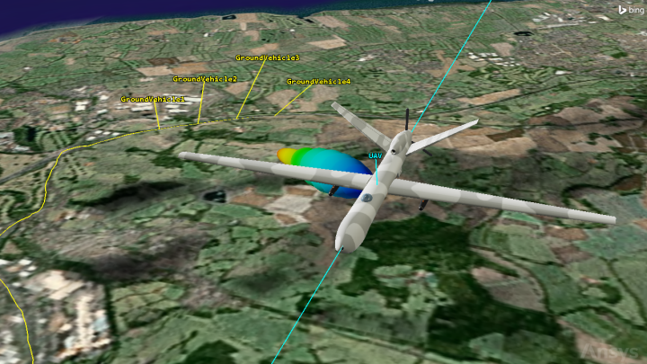
UAV Parabolic Antenna Pattern Tracking GroundVehicle2
Note the antenna gain volume for the UAV's receiver as it tracks the reported location of GroundVehicle2.
Viewing the convoy's route
In addition to aircraft, the STK application also offers propagators for high-fidelity modeling of
- Right-click on GroundVehicle2 () in the Object Browser.
- Select Zoom To in the shortcut menu.
- Use your mouse to zoom out until you can see the entire convoy.
- Click Start () to view the animation.
- Click Reset (
 ) when you are finished.
Watch as the convoy exits the motorway and heads into the mountains.
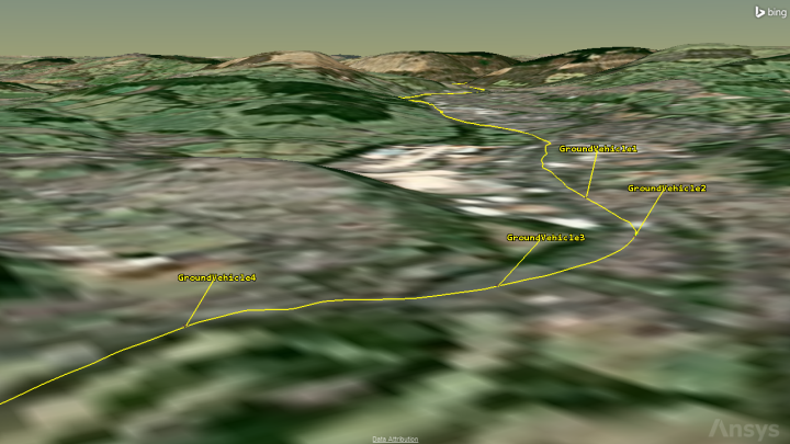
Convoy En Route
Understanding the convoy's communications system
The second vehicle in the convoy is serving as a mobile command and control center. It is connected to the UAV through a targeted 14-gigahertz parabolic antenna and to the other vehicles in the convoy through a 2.4-gigahertz wireless network.
Understanding the convoy's connection to the UAV
View the communications vehicle's UAV antenna system.
- Open GV2toUAV's () Properties ().
- Select the Basic - Pointing page when the Properties Browser opens.
- Note the Pointing Type is Targeted.
- Click to close the Properties Browser without making any changes.
- Open GV2toUAVantenna's () Properties ().
- Select the Basic - Definition page when the Properties Browser opens.
- Note the following design specifications:
- Click to close the Properties Browser without making any changes.
Note the ground vehicle's sensor is targeted to the UAV.
| Option | Value |
|---|---|
| Design Frequency | 14 GHz |
| Diameter | 9.75 in |
| Efficiency | 55 % |
Viewing the transmitter specifications
A
- Open GV2toUAV_Xmtr's (
 ) Properties ().
 - Select the Basic - Definition page when the Properties Browser opens.
- Note the Transmitter model is set to Complex Transmitter Model.
- Select the Model Specs tab.
- Note following model specs:
- Select the Antenna tab.
- Note the transmitter is linked to Sensor/GV2toUAV/Antenna/GV2toUAVantenna.
- Click to close the Properties Browser without making any changes.
A
| Option | Value |
|---|---|
| Frequency | 14 GHz |
| Power | -10 dBW |
Understanding the convoy's WiFi antennas
The vehicles in the convoy use dipole antennas for their communications.
- Open WiFi2's () Properties ().
- Select the Basic - Definition page when the Properties Browser opens.
- Note that Dipole is selected for the Antenna Model.
- Note the following design specifications:
- Click to close the Properties Browser without making any changes.
| Option | Value |
|---|---|
| Design Frequency | 2.4 GHz |
| Length/Wave Length Ratio | 1 |
| Efficiency | 100 % |
The convoy's WiFi antennas are named as follows:
| Object | Antenna Name |
|---|---|
| GroundVehicle1 | WiFi1 |
| GroundVehicle2 | WiFi2 |
| GroundVehicle3 | WiFi3 |
| GroundVehicle4 | WiFi4 |
Viewing the communication vehicle's antenna patterns
View the communication vehicle's antenna patters in the 3D Graphics window.
- Zoom back in to GroundVehicle2 ().
- Click Start () in the Animation toolbar to animate the scenario.
- Click Reset () when you are finished.
Note the antenna gain volumes for GroundVehicle2. The parabolic antenna pattern looks very similar to that on the UAV and rotates to target the UAV. The dipole antenna pattern is static. You will notice that both antenna patterns originate from the roof of the vehicle. In the case of the GV2toUAVantenna, its parent GV2toUAV Sensor object's
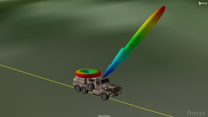
GroundVehicle2 Antenna Patterns
Analyzing the UAV communications link
The STK application allows you to determine the times one object can "
The Scalable Networks Modeling Interfaces leverages access availability between two link antennas based on all active constraints. If the STK application determines that there is no access between the two antennas, the STK application tells Scalable Networks Modeling Interface that communication is not possible.
Computing access
Before you can evaluate the quality of the communications link, you must first compute access between the convoy's transmitter and the UAV's receiver using the
- Right-click on GV2toUAV_Xmtr () in the Object Browser.
- Select Access... (
 ) in the shortcut menu.
 - Expand (
 ) UAV () in the associated objects list when the Access tool opens.
 - Select UAVtoGV2_Rcvr ().
- Click
 .
.
Creating a dynamic data display
You can
- Click .
- Click when the 3D Graphics Data Display dialog box opens.
- Select Link Budget - BER in the Styles list when the Add a Data Display dialog box opens.
- Click to confirm your selection and to close the Add a Data Display dialog box.
- Click to confirm your changes to close the 3D Graphics Data Display dialog box.
- Keep the Access tool open.
The
Viewing the dynamic data display
View the dynamic data display in the 3D Graphics window.
- Bring the 3D Graphics window to the front.
- Click Start () in the Animation toolbar to view the dynamic display of data.
- Click Reset () when you are finished.
Generating a static link budget report
You can also determine the quality of the link between the UAV and the convoy by generating a static Link Budget - Detailed report. A
- Bring the Access tool to the front.
- Click .
- Make sure that GroundVehicle-GroundVehicle2-Transmitter-GV2toUAV_Xmtr-To-Aircraft-UAV-Receiver-UAVtoGV2_Rcvr (
 ) is selected in the Object List when the Report & Graph Manager opens.
 - Select the Link Budget- Detailed (
 ) report in the Installed Styles (
 ) folder in the Styles list.
 - Click .
Reviewing the Link Budget- Detailed report
Once the report opens, review the report.
- Scroll through the report.
- Right-click on the Mission Area 3D Graphics window tab at the bottom of the STK workspace.
- Select Close All But This in the shortcut menu.
- Save (
 ) your scenario.
Notice that the BER remains negligible throughout the analysis.
Opening the Scalable Networks Modeling Interface for STK Communications plugin
The STK application's Communications capability offers an enhanced solution for communications network modeling by introducing off-the-shelf interoperability with the EXata network modeling software, an industry-recognized network modeling and simulation tool, which enables you to evaluate on-the-move communication networks: the
The Scalable Networks Modeling Interface can be accessed through the Scalable Networks Modeling Interface toolbar; with the toolbar, you can configure your EXata scenario, run experiments, and display statistical charts.
- Select Toolbars in the View menu.
- Select Scalable Networks Modeling Interface from the View menu to display the Scalable Networks Modeling Interface toolbar.

Scalable Networks Modeling Interface functions are also available from the Scalable Networks Modeling Interface submenu in the Utilities menu.
The Scalable Networks Modeling Interface features the ability to display and animate event types, such as Receive, Unicast, and Drop, which are published by the EXata simulation. You can animate the events using the buttons on the Scalable Networks Modeling Interface toolbar. Animation events are beyond the scope of this tutorial.
Opening the Scalable Networks Modeling Interface Configuration File Scenario Explorer
The Scalable Networks Modeling Interface
- Click Scenario Explorer (
 ) on the Scalable Networks Modeling Interface toolbar.
 - Expand (
 ) ScalableNetworksInterface (
 ) in the object tree when the Scalable Networks Modeling Interface Scenario Explorer window opens.
Reviewing the scenario's General Settings
Now that the physical objects are fully defined using the STK software, you can map those objects into a EXata simulation. Use the Scalable Networks Modeling Interface Scenario Explorer to define your scenario's configuration.
- Expand () the Scenario Configuration (
 ) folder.
 - Expand () General (
 ).
). - Select General Settings ().
- Review the properties panel.
Notice that the Simulation Time of 2400S (equivalent to 40 minutes) is inherited from the STK Scenario Analysis time. Also, notice that the 2400S Simulation Time is bolded. All values that are user-defined or inherited from the STK software are bolded. Take note as well that the default Experiment Name is exata.
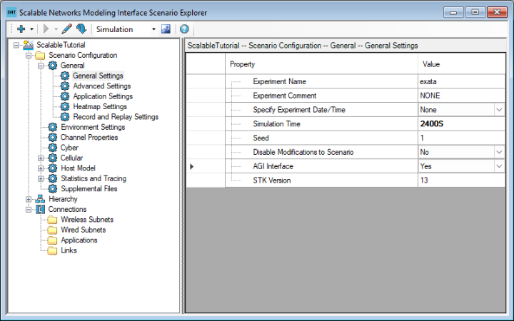
Scenario Settings
Enabling the Statistics Database
One of the powerful tools the EXata software provides is for the generation of numerous tables of statistics through its Statistics Database. The Statistics Database collects time-based statistics at a high level of granularity during a network simulation. The statistics captured in the database's tables can be analyzed and used to generate reports to understand network performance issues at a much finer level of detail than you can with just the STK software itself. In this case, you want to use the Statistics Database to collect data on the transmission and reception of individual signals sent over the network's PHY layer.
- Expand () Statistics and Tracing ().
- Select Statistics Database ().
- Open the Enable Statistics Database - Value drop-down list.
- Select Yes.
- Note the Engine Type property is set to SQLite.
- Expand () the Statistics Database Detail Level - Events Tables property.
- Select Yes for the PHY Signal Events Table property.
The child properties of Enable Statistics Database should expand out automatically.
The Scalable Networks Modeling Interface supports the creation of SQLite and MariaDB database files.
This will expand the PHY Signal Events Table property to show its child properties.
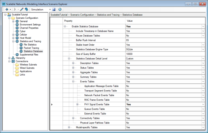
Statistics Database Properties
Now, when you run your experiment, an SQLite-compatible database file with the selected tables and columns will be generated.
Adding another channel
Your network operates on two channels: a 2.4-gigahertz wireless channel for the convoy is already present, but you need to add a second, 14-gigahertz channel for communications between GroundVehicle2 and the UAV.
- Select Channel Properties () in the Scenario Configuration () folder.
- Click in the Value field for Number of Channels.
- Enter 2 in the Value field for Number of Channels.
- Select the Enter key.
- Note that the Channel Name [1] property is automatically set to channel1.
- Enter 14 GHz in the Channel Frequency [1] - Value field.
- Select the Enter key.
- Leave the channels names set to their default values.
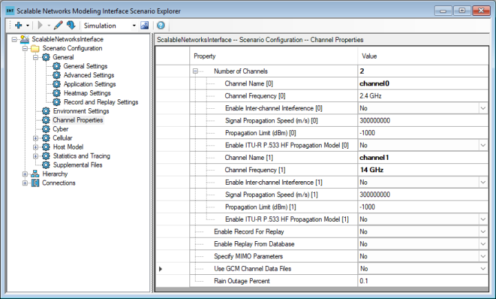
Channel Properties
Reviewing the scenario hierarchy
A scenario hierarchy is composed of nodes. Nodes communicate with each other through connected network interfaces. Each node must have at least one network interface for it to be considered in the network analysis. Verify that there is one node for each STK parent object in the STK scenario hierarchy.
- Expand () Hierarchy (
 ) in the object tree.
 - Select UAV ().
- Ensure there is one Node ID listed in the properties panel.
- Repeat the process for GroundVehicle1 (), GroundVehicle2 (), GroundVehicle3 (), and GroundVehicle4 ().
- Confirm your Node IDs match the following table:
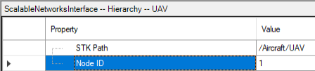
Object Nodes
| Node | Node ID |
|---|---|
| UAV | 1 |
| GroundVehicle1 | 2 |
| GroundVehicle2 | 3 |
| GroundVehicle3 | 4 |
| GroundVehicle4 | 5 |
Defining network interfaces
A
Renaming an existing interface
By default, objects that already have antennas attached to them in your STK scenario automatically have a wired and a wireless interface created for them. The wireless interfaces are already configured to use the attached Antenna objects. These interfaces are listed in a nested Interfaces folder for each node in the Scenario Hierarchy. For clarity of organization, begin by renaming the existing wireless interface for the UAV node.
- Expand () UAV () in the object tree.
- Expand () the Interfaces () folder.
- Note that UAV () has two network interfaces (
 ): interface0 () and interface1 ().
 - Right-click on interface1 ().
- Select Edit in the shortcut menu.
- Enter UAVtoGV2 in the Interface Name field when the Edit Wireless Interface dialog box opens.
- Note that UAVtoGV2/UAVtoGV2_Antenna is automatically selected for the Transmit Antenna - Instance Name.
- Also note that the Use Transmit Antenna for Receive check box is automatically selected in the Receive Antenna panel.
- Click to confirm your changes and to close the Edit Wireless Interface dialog box.
interface0 () is the default wired interface; interface1 () is the default wireless interface.
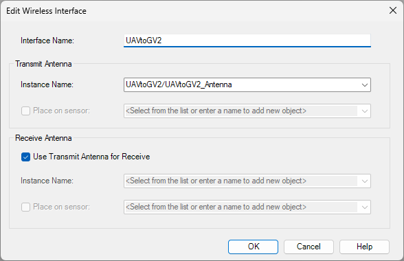
Edit Wireless Interface
You can control whether wired and wireless interfaces are created by default when an object is added to your scenario by updating the
Renaming the remaining wireless interfaces
Repeat the process for each ground vehicle's default wireless interface.
- Expand () each of the four GroundVehicle () nodes.
- Expand () the Interfaces () spellfolder nested under each of the ground vehicle () nodes.
- Note that GroundVehicle2 () has three default interfaces (): one wired connection and one wireless connection for each attached antenna.
- Repeat the steps in the previous section to rename each ground vehicle node's default wireless interfaces (), as specified below:
| Node | Default Interface Name | New Interface Name | Instance Name |
|---|---|---|---|
| GroundVehicle1 | interface1 | GV1_WiFi | WiFi1 |
| GroundVehicle2 | interface1 | GV2_WiFi | WiFi2 |
| interface2 | GV2toUAV | GV2toUAV/GV2toUAV_Antenna | |
| GroundVehicle3 | interface1 | GV3_WiFi | WiFi3 |
| GroundVehicle4 | interface1 | GV4_WiFi | WiFi4 |
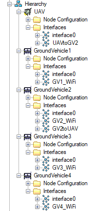
Interface Hierarchy
) the wireless interfaces (), you will note that they have properties for the Physical Layer, MAC Layer, and other network layers. For this tutorial, you don't need to define them at the interface level, since you will be defining them at the subnet level and those definitions will take precedence.Creating network connections
Now that you have defined the interfaces between STK antennas, you can define your connections. The Scalable Networks Modeling Interface enables you to
Creating the wireless subnet between the ground vehicle and the UAV
A
- Right-click on Connections (
 ) in the object tree.
 - Select Add Wireless Subnet ... in the shortcut menu.
- Enter GV2toUAV in the Name field when the Add Wireless Subnet dialog box opens.
- Move () UAV/UAVtoGV2 from the Available Interfaces list to the Selected Interfaces list.
- Move () GroundVehicle2/GV2toUAV to the Selected Interfaces list.
- Select the Assign IP address to interfaces to match network IP check box.
- Keep the default values for all other parameters.
- Click to confirm your changes and to close the Add Wireless Subnet dialog box.
If you do not select the Assign IP address to interfaces to match network IP check box, the Scalable Networks Modeling Interface will not run.
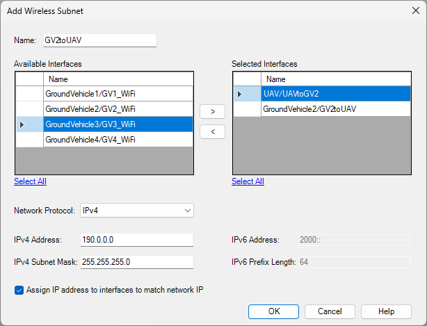
Add Wireless Subnet
Setting up the GV2toUAV wireless subnet's channel properties
Set up the GV2toUAV wireless subnet so that it can only transmit and receive on the 14-gigahertz channel. The GV2toUAV wireless subnet is located in the Connections - Wireless Subnets folder in the object tree.
- Expand () Connections () in the object tree.
- Expand () the Wireless Subnets () folder.
- Expand () GV2toUAV (
 ).
). - Select Physical Layer ().
- Click on the Listenable Channel Mask - Value field.
- Clear the Enabled? check box for the channel 0 - 2.4 GHz Frequency option when the Channel Mask Editor dialog box opens.
- Select the Enabled? check box for the channel 0 - 14 GHz Frequency option.
- Click to confirm your change and to close the Channel Mask Editor dialog box.
- Set the Listening Channel Mask to use channel1 by selecting only 14 GHz in the Channel Mask Editor.
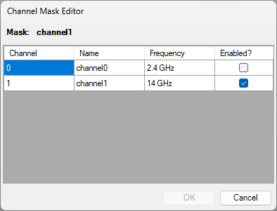
Channel Mask Editor
Note that the Listenable Channel Mask - Value has been set to channel1; channel1 is the default name of your 14 GHz channel.
Configuring the subnet's PHY layer
Select a Radio Type that is appropriate for the large range of the link between the Ground Vehicle and the UAV. Use an Abstract radio type and update its properties. The Scalable Networks Modeling Interface interacts with the PHY layer's transmit power, frequency, and data rate to compute the received signal-to-noise ratio and BER based on the received power computed by the STK application.
- Open the Radio Type drop-down list in the properties panel.
- Select Abstract.
- Expand () the Tx and Rx Use Same Frequency property.
- Set the Tx and Rx Center Frequency - Value to 14 GHz.
- Set the Rx Bandwidth - Value to 32 MHz.
- Expand () the Number of Modulation and Coding Schemes property.
- Set the Data Rate [0] - Value to 16 Mbps.
- Set the Frequency Bandwidth [0] - Value to 32 MHz.
Setting the Reception Sensitivity and Threshold
For the purposes of your network test, you want to examine the receiver sensitivity and threshold values.
- Set the Reception Sensitivity (dBm) [0] - Value to -40.
- Set the Reception Threshold (dBm) [0] - Value to -50.
When working with EXata, the reception threshold should be set lower than the sensitivity.
Your Physical Layer properties should match the following table:
| Property | Value |
|---|---|
| Listenable Channel Mask | channel1 |
| Listening Channel Mask | channel1 |
| Radio Type | Abstract |
| Tx and Rx Center Frequency | 14 GHz |
| Rx Bandwidth | 32 MHz |
| Data Rate [0] | 16 Mbps |
| Frequency Bandwidth [0] | 32 MHz |
| Reception Sensitivity (dBm) [0] | -40 |
| Reception Threshold (dBm) [0] | -50 |
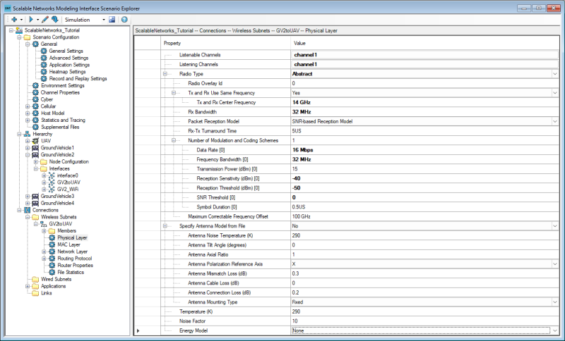
Wireless Subnet Physical Layer configuration
Setting up the MAC layer
Use a generic MAC protocol for the wireless interface.
- Select MAC Layer () in the object tree.
- Open the MAC Protocol - Value drop-down list.
- Select Generic MAC.
Setting up the Network layer
Configure the network's buffer to use a single IP output queue.
- Expand () Network Layer () in the object tree.
- Select Schedulers and Queues ().
- Set the Number of IP Output Queues - Value to 1.
- Leave all other values their defaults.
Setting up the Routing Protocol
Use the Ad hoc On-Demand Distance Vector Routing (AODV) network protocol, which is efficient for dynamic, rapidly changing topologies.
- Select Routing Protocol () in the object tree.
- Select AODV in the Routing Protocol IPv4 - Value drop-down list.
- Leave all other values their defaults.
Creating and configuring the convoy's wireless subnet
Now, add and configure a wireless subnet for the convoy.
- Right-click on Connections () in the object tree.
- Select Add Wireless Subnet ... in the shortcut menu.
- Set the following properties when the Add Wireless Subnet dialog box opens:
- Select the Assign IP address to interfaces to match network IP check box.
- Click to confirm your changes and to close the Add Wireless Subnet dialog box.
- Configure the Convoy's wireless subnet Physical Layer () as follows:
- Set the Network Layer's () Schedulers and Queues () Number of IP Output Queues to 1.
- Set the Routing Protocol () Routing Protocol IPv4 to AODV.
| Name | Selected Interfaces |
|---|---|
| Convoy | GroundVehicle1/GV1_WiFi |
| GroundVehicle2/GV2_WiFi | |
| GroundVehicle3/GV3_WiFi | |
| GroundVehicle4/GV4_WiFi |
Keep the default values for all other parameters.
Remember that, as when you set up the previous wireless interface, if you do not select the Assign IP address to interfaces to match network IP check box, the Scalable Networks Modeling Interface will not run.
| Property | Value |
|---|---|
| Listenable Channel Mask | channel0 |
| Listening Channel Mask | channel0 |
| Radio Type | 802.11b Radio |
| Transmission Power at 1 Mbps (dBm) | 45 |
| Transmission Power at 2 Mbps (dBm) | 45 |
| Transmission Power at 5.5 Mbps (dBm) | 45 |
| Transmission Power at 11 Mbps (dBm) | 45 |
Creating a CBR application link
An
- Right-click on Connections () in the object tree.
- Select Add Application ... in the shortcut menu.
- Open the Source drop-down menu when the Add Application dialog box opens.
- Select GroundVehicle4.
- Open the Destination drop-down list.
- Select UAV.
- Set the Application type to CBR.
- Click to confirm your changes and to close the Add Application dialog box.
This option sends data from a client to a server at a constant bit rate (CBR).
Setting up the CBR application
Configure the items for the CBR application to send and its Start and End times.
- Expand () the Applications () folder, located under Connections (), in the object tree.
- Select CBR: GroundVehicle4 --> UAV (
 ).
). - Set the following properties for the CBR application:
| Parameter | Value |
|---|---|
| Items to Send | 360 |
| Start Time | 790 seconds |
| End Time | 1150 seconds |
The Start Time and End Time settings enable you to focus on just a small portion of the route. The Items to Send value of 360, in combination with the 360-second time period between Start Time and End Time, force the application to send one packet per second.
Running a Scalable Networks Modeling Interface experiment
Apply all network settings and compute network-level statistics on your STK scenario by running an experiment, then view the results.
Running your experiment
You can run the experiment through the Scalable Networks Modeling Interface Scenario Explorer toolbar.
- Ensure Simulation is selected in the drop-down list on the Scenario Explorer toolbar.
- Click Run Experiment (
 ) on the Scenario Explorer toolbar.
 - Take note of the Initializing status displayed on the bottom left of the Simulator Run Control window when it opens.
- When the status has changed to Ready to Run, click .
- When the simulation is completed the Stat File viewer will automatically open.
You can choose whether you are performing a network simulation or network emulation.
Initialization can take anywhere from several seconds to several minutes, depending on the complexity of your scenario and experiment.
The elapsed Simulation Time is displayed, and the status of the run is displayed in the Progress bar.
Each time you run a Scalable Networks Modeling Interface experiment, the STK application populates a working directory with files used by Scalable Networks Modeling Interface. The STK application also places the Stat file into this folder.
The folder structure is:
<user-selected folder or STK scenario folder>\Scalable Networks Modeling Interface Experiments\<Scalable Networks Modeling Interface experiment name>\<date in format YYYY_MM_DD>\<time in format HH_MM_SS>
An example is:
C:\Users\<username>\Documents\STK_ODTK 13\ScalableTutorial\Scalable Networks Modeling Interface Experiments\exata\2026_03_05\09_32_33.
In addition to the Stat file, the following Scalable Networks Modeling Interface Experiment files will be saved to that working directory, which is specified in the Scalable Networks Modeling Interface preferences:
- Application configuration file (*.app), which specifies the applications running on the nodes in the scenario and is referenced by the scenario configuration file.
- Scenario configuration file (*.config), which is the primary input file for the Scalable Networks Modeling Interface application and specifies the network scenario and parameters for the simulation. This file allows you to map the interfaces to their respective antennas and can be used directly in the EXata software itself.
- Qimap file (*.qimap), which contains the mapping between STK objects and the Scalable Networks Modeling Interface nodes and is required by both the STK and the EXata applications.
- STK VDF file (*.vdf), which enables you to view the exact settings used by STK software when generating the Scalable Networks Modeling Interface stat file. This is a handy reference if you plan to later change the STK scenario. Be aware that each copy of an STK scenario can potentially use a large amount of disk space.
The folder may also contain:
- Generic database file (*.db), built using SQLite, if you specified one to be generated in the Statistics Database properties earlier
- log file (*.log), containing link and node information
- JSON file (*.json), containing structured data about your scenario
You can see a visual representation of this workflow here.
Viewing the Command-line Output Log
Before taking a close look at the Stat File viewer, it is helpful to review the Command-line Output Log, which lists all messages generated by the Scalable Networks Modeling Interface Experiment run. If you ever need to debug your scenario or determine why your experiment hasn't initialized or run successfully, the Command-line Output Log will show you that information.
- Return to the Scalable Networks Modeling Interface Scenario Explorer window.
- Click Simulator Command-line Output Log (
 ) on the Scenario Explorer toolbar.
 - Correct any errors (
 ) listed in the log to run your experiment successfully, if necessary.
 - Re-run () the Scalable Networks Modeling Interface experiment, if necessary.
Analyzing your experiment
With your experiment completed, review the results to understand any network issues that may exist with your network configuration or scenario.
Reviewing the Stat file
Statistics (or Stat) files are the primary output file generated by a Scalable Networks Modeling Interface simulation run and have a *.stat file extension. When a simulation run is completed, a Stat file is automatically loaded into the Stat File viewer.
You can also import a EXata Stat file for review in the STK application by clicking Import Results ( ) on the Scenario Explorer toolbar.
- Take note of the categories listed in the object tree.
- Select the Physical - Abstract - Signals Transmitted (signals) category.
- Note the results on the Physical - Abstract bar chart.
- Hover over the results to show the Node, the Interface, and the number of packets sent.
- Select the Network - AODV for IPv4 - Number of Data Packets Dropped for no route category.
- Review the Network - AODV for IPv4 chart.
These include Throughput, Broadcasts Sent and Received, Packets Queued, Packets dropped, Route Timeouts, and Packet Times. Graphs are shown by node ID (interface ID). The Statistics file is the primary output file generated by a Scalable Networks Modeling Interface simulation run. The statistical categories are listed in the object tree, including Throughput, Broadcasts Sent and Received, Packets Queued, Packets dropped, Route Timeouts, and Packet Times. Graphs are shown by node ID (interface ID).
You can click on any parameter in the Stat File viewer to display its statistics from the simulation run.
As expected, GroundVehicle2 is sending out a lot of signals, as it is the main communications hub. However, you configured your experiment to send 360 packets of information, and only 219 packets were received by the UAV.
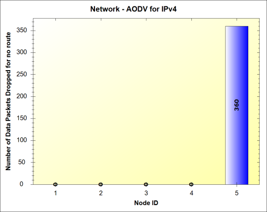
All data packets dropped
If you want to export an image of a chart for sharing outside of the STK application, you can right-click on the chart and select Save Image As... in the shortcut menu.
Recall the goal of your experiment was to use a CBR application to send data from GroundVehicle4 to the UAV. However, all 360 packets of information for Node ID 5 (which corresponds to GroundVehicle4) were dropped for no route. Another clue that your network isn't performing as expected is under the Application category; you can see categories for the CBR Client, but no categories for CBR Server, which means you are not getting any server-side results.
Since your BER was negligible throughout the scenario, there must be some other cause for the lost data. You will need to investigate your results in greater detail to understand why the signals aren't being sent.
Reviewing the Statistics Database
The Stat file can only tell you so much. To help identify the root cause of the network performance issues, examine the SQLite database file you configured to be produced in the Scenario's Statistics Database properties.
Opening the database file
Explore the database file with the database inspection tool of your choice. Examples include DB for SQLite or the MATLAB platform's Database Explorer app.
- Open Windows File Explorer.
- Navigate to your scenario folder (for example, C:\Users\<username>\Documents\STK_ODTK 13\ScalableTutorial).
- Open the exata sub-folder.
- Open the folder with today's date.
- Open the folder with the most recent time.
- Open the database (*.db) file with the database inspection tool of your choice.
Reviewing the physical events data
Recall that you configured your experiment to capture details about events with the physical layer. Review the PHY_Events table to learn more about the specifics of your network's performance.
- If you are using the DB for SQLite software, select the Browse Data tab.
- Open the PHY_Events table.
- Browse through the data in the table.
- Review the data in FailureType column.
- Sort the data in the SignalPower column from the smallest value to the largest value.
- Review the data in the SignalPower column.
- Leave your database inspection tool and Windows File Explorer open.
Other applications may have different interface options.
You can see through the various columns the various properties of the messages that have been sent.
As you scroll through the data in the column, you can see there are many instances where the FailureType is Signal below Rx Sensitivity. This is a clue why your packets are being dropped.
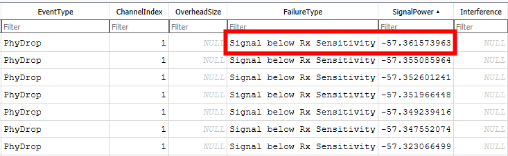
Sorted db file showing weakest signal
You can see that the weakest signal was around -57 decibel-milliwatts, and for signals of that magnitude, you encountered a PhyDrop EventType, with a FailureType of Signal below Rx Sensitivity. From these data, you can see that you need a more sensitive receiver in order to receive signals at least as weak as -57 decibel-milliwatts.
Updating your scenario and re-running your experiment
Recall that you had previously set reception sensitivity and threshold values of -40 decibel-milliwatts and -50 decibel-milliwatts, respectively. Increase these values to allow the signals to be received, the re-run your experiment.
Updating the GV2toUAV wireless subnet's settings
Increase the reception sensitivity and threshold values for your experiment.
- Return to the STK application.
- Go to the Scalable Networks Modeling Interface Scenario Explorer window.
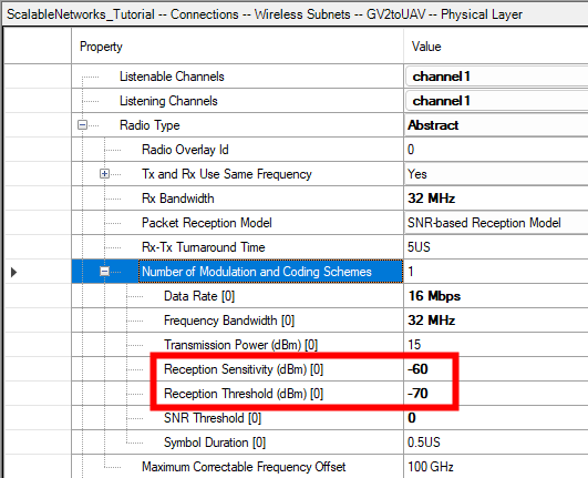
- Select Connections - Wireless Subnets - GV2toUAV - Physical Layer () in the object tree.
- Expand () the Number of Modulation and Coding Schemes property.
- Set the Reception Sensitivity (dBm) [0] - Value to -60.
- Set the Reception Threshold (dBm) [0] - Value to -70.
- Save () your scenario.
Updated sensitivity and threshold values
Re-running your experiment and reviewing the results
Now that you've set your values, run your experiment again and review the data
- Click Run Experiment () on the Scenario Explorer toolbar.
- When the status has changed to Ready to Run, click .
- Review the data when the Stat File viewer open.
- Select the Network - AODV for IPv4 - Number of Data Packets Received category.
- Review the Network - AODV for IPv4 chart.
- Note also that you now have server-side results you can explore through the Application - CBR Server properties.
The progress bar may show 100% before the experiment fully initializes; this is left over from your previous run, it will clear once your experiment is ready to run.
You can see that unlike in your previous experiment, there is no longer category for Network - AODV for IPv4 - Number of Data Packets Dropped for no route category.
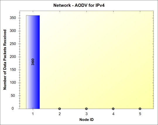
All packets received
Note that Node ID 1 (UAV) has now received all 360 data packets.
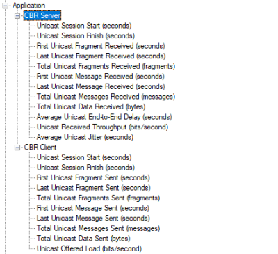
CBR Server categories present
Confirming the changes in the database file
The statistics look good, but you can also review the database file created from your latest run to confirm.
- Return to Windows File Explorer.
- Navigate up to the date sub-folder.
- Open your most recent experiment folder.
- Open the database (*.db) file with the database inspection tool of your choice.
- If you are using the DB for SQLite software, select the Browse Data tab.
- Open the PHY_Events table.
- Sort the data in the SignalPower column from the smallest value to the largest value.
- Review the data in the SignalPower column.
- Close your database inspection tool.
Your updated database file is in a new experiment folder.
Now, the FailureType column for the lowest signal powers have a null value, and instead of a PhyDrop event type, the lowest SignalPower values are associated with reception and transmission events. The data confirm you've successfully adjusted your reception sensitivity and threshold to receive all the signals.
Exporting your experiment
Once you are happy with your results, export your experiment.
- Click the down arrow next to Run Experiment (
 ).
). - Select Export Experiment in the drop-down menu.
- Read the warning when the Experiment Export dialog box opens.
- Click to close the Experiment Export dialog box and to open the containing folder.
- Close Windows File Explorer.
Importing an EXata scenario using a Scalable Networks Modeling Interface Configuration File
An alternative method to configuring your experiment in the STK application is to import the wireless interfaces from an EXata scenario directly into the STK application through the Scalable Networks Modeling Interface. The
A sample configuration file generated by the EXata software is included in your scenario and can be found in your scenario folder. Though a *.config file is also generated by the Scalable Networks Modeling Interface when you run an experiment, only those created by EXata proper can be ingested by the Configuration File Importer.
You can configure a scenario built in the EXata software for use with the STK application. Once you have everything configured the way you like, you must save it to produce a *.config file.
- In the EXata application, select the File menu.
- Select Save As Portable....
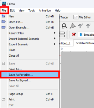
Save As Portable option in the EXata software
This option will create a *.config file, which you can then import into your STK application using the Scalable Networks Modeling Interface Configuration File Importer.
Importing a configuration file using the Scalable Networks Modeling Interface Configuration File Importer
Open the Scalable Networks Modeling Interface Configuration File Importer to bring in the configuration file included with your scenario.
- Click Configuration File Importer (
 ) on the Scalable Networks Modeling Interface toolbar.
 - Click Add Configuration File (
 ) on the Configuration File Importer toolbar when the Scalable Networks Modeling Interface Config Importer window opens.
 - Navigate to your scenario folder when the Open dialog box opens.
- Select ScalableNetworks_Tutorial.config.
- Click to confirm your selection and to close the Open dialog box.
- Note that ScalableNetworks_Tutorial.config is now listed in the Simulator Configuration File panel.
- Also note that ScalableNetworks_Tutorial.config has a warning (
 ) status and the Run Experiment button is grayed out.
You still need to map all your interfaces to your STK antenna objects before you can run an experiment.
Mapping the wireless interfaces to the STK antennas
View all the available interfaces and map them to their respective STK Antenna objects.
- Right-click on UAV (1) () in the Available Wireless Interfaces tree.
- Select Unmapped Interfaces in the shortcut menu.
- Select Expand in the Unmapped Interfaces submenu.
- Right-click on UAV () in the Available Antenna Objects tree.
- Select Expand All.
- Click and Drag 190.0.0.1 () onto UAVtoGV2_Antenna ().
- Using the same procedure as 190.0.0.1, make the following mappings:
The numbers in the parentheses are the Node IDs.
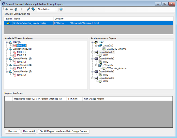
Config Importer
Note that a green check box appears over 190.0.0.1 () and the mapping has been added to the table in the Mapped Interfaces panel.
| Wireless Interface | Antenna Object |
|---|---|
| 190.0.0.2 | GV2toUAV_Antenna |
| 190.0.1.1 | WiFi1 |
| 190.0.1.2 | WFi2 |
| 190.0.1.3 | WiFi3 |
| 190.0.1.4 | WiFi4 |
If you have trouble identifying the wireless interfaces by their IP addresses, you can review the addresses and their node assignments in the EXata application's Table View.
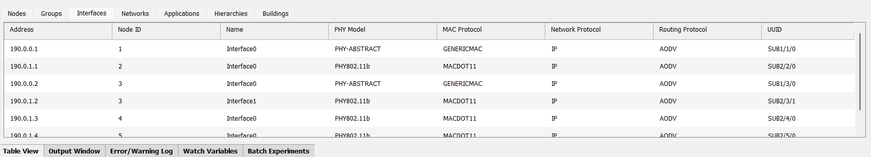
EXata Table View
Once all of your mappings are completed, the status for the simulator configuration file will be updated with a green check mark ( ) to indicate that the configuration file is up-to-date and all interfaces are mapped to STK antenna objects. The Run Experiment () button will also become active and you can then proceed to run your simulation as before.
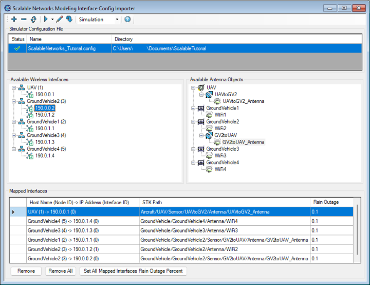
Config Importer: All interfaces mapped
Saving your work
Clean up your workspace and close out your scenario.
- Close the Stat File Viewer, the Scalable Networks Modeling Interface Scenario Explorer, and all reports and windows except the 3D Graphics window.
- Save () your work.
- Close your scenario when you are finished.
Summary
You opened a preconfigured VDF file, and saved it as a Scenario file. The scenario used STK software's Communications capability to model a communications network between a convoy of ground vehicles traversing mountainous terrain and a UAV flying overhead. External ephemeris files were used to model the vehicles' routes and an attitude file was used to model the UAV's flight dynamics. You calculated access between the convoy and the UAV, then evaluated the quality of the link using a preinstalled report in the Report & Graph Manager. You then used Scalable Networks Modeling Interface to leverage your STK scenario with the EXata software's physical layer modeling capabilities to configure wireless network communications interfaces. You then performed an experiment on your network and analyzed the results. You examined the experiment's results and used them to improve your network performance. Finally, you imported a configuration file and used the Scalable Networks Modeling Interface Configuration File Importer to create mappings between an EXata scenario and STK antenna objects. By using the Scalable Networks Modeling Interface, you were able to combine the strengths of both the STK software and EXata network modeling software to evaluate your communications links.