Part 9:
STK Pro, STK Premium (Air), STK Premium (Space), or STK Enterprise
You can obtain the necessary licenses for this tutorial by contacting AGI Support at support@agi.com or 1-800-924-7244.
The results of the tutorial may vary depending on the user settings and data enabled (online operations, terrain server, dynamic Earth data, etc.). It is acceptable to have different results.
Capabilities covered
This lesson covers the following capabilities of the Ansys Systems Tool Kit® (STK®) digital mission engineering software:
- STK Pro
- Analysis Workbench
- Volumetric Analysis
Problem
Engineers and operators require a quick way to determine if the Earth, local terrain, nature, and man-made structures affect visibility between ground sites and satellites for a variety of purposes, such as communications, imaging, radar, and general situational awareness. A country's space program is planning to install a satellite tracking radar in an area that has distant hills and a large mountain range. A communication antenna, enclosed by a large radome, will be constructed close by. You want to determine how much impact the Earth, terrain and the radome will have on the radar's field of view.
Solution
Using the STK software, insert Facility objects to simulate the radar and communications sites. Use a local terrain file for analysis and determine access times between the radar's field of view and several Earth-observing satellites. Use the AzEl Mask tool to determine if the communications site's radome further degrades the radar's access times to the satellites. Insert an Area Target object to outline the approximate maximum distance that a satellite can be observed by the radar site. Use the Analysis Workbench capability's Spatial Analysis tool and the Volumetric Analysis capability to build and analyze a Volumetric object to determine how much of the radar's field of view is blocked by the Earth, terrain, and the radome at a specified distances and altitudes.
What you will learn
Upon completion of this tutorial, you will understand the following:
- How to use the AzEl Mask tool
- How to use the Analysis Workbench capability’s Time tool and Spatial Analysis tool
- How to use the Volumetric Analysis capability and Volumetric objects
Video guidance
Watch the following video. Then follow the steps below, which incorporate the systems and missions you work on (sample inputs provided).
Creating a new scenario
Create a new scenario, then build from there.
- Launch the STK application (
 ).
). - Click
 Create a Scenario in the Welcome to STK dialog box.
 - Enter the following in the STK: New Scenario Wizard:
- Click when you finish.
- Click Save (
 ) when the scenario loads. The STK application creates a folder with the same name as your scenario in the location specified above.
 - Verify the scenario name and location.
- Click .
| Option | Value |
|---|---|
| Name | AzElMask_Volumetrics |
| Location | Default |
| Start | 15 Mar 2024 12:00:00.000 UTCG |
| Stop | + 1 day |
Save (![]() ) often!
) often!
Turning off streaming terrain
Since you will use a local analytical terrain file in this analysis, disable Terrain Server.
- Right-click on AzElMask_Volumetrics's () in the Object Browser.
- Select Properties (
 ).
). - Select the Basic - Terrain page.
- Clear the Use terrain server for analysis check box in the Terrain Server panel.
- Click to accept the change and close the Properties Browser.
Adding analytical and visual terrain
Load
- Bring the 3D Graphics window to the front.
- Click Globe Manager (
 ) in the 3D Graphic window's Globe Manager toolbar.
 - Click Add Terrain/Imagery (
 ) in the Globe Manager Hierarchy toolbar when Globe Manager opens.
 - Select Add Terrain/Imagery... (
 ) in the drop-down menu.
 - Click the Path ellipsis (
 ) when the Globe Manager: Open Terrain and Imagery Data dialog box opens.
 - Navigate to <Install Dir>\Data\Resources\stktraining\imagery (for example, C:\Program Files\AGI\STK_ODTK 13\Data\Resources\stktraining\imagery) in the Select Image Directory list when the Browse For Folder dialog box opens.
- Click to select the directory and to close the Browse For Folder dialog box.
- Select the check box for RaistingStation.pdtt.
- Click .
- Click to enable terrain for analysis and to close the Use Terrain for Analysis prompt.
Decluttering the 3D Graphics window labels
Enable
- Bring the 3D Graphics window to the front.
- Click Properties (
 ) in the 3D Window Defaults toolbar.
 - Select the Details page.
- Select the Enable check box in the Label Declutter panel.
- Click to confirm your selection and to close the Properties Browser.
Modeling the radar site
The radar site is located in the Alpine Foreland in Southern Germany.
Inserting a new Facility object
Use a Facility object to model the radar site.
- Bring the Insert STK Objects tool (
 ) to the front.
 - Select Facility (
 ) in the Select An Object To Be Inserted list.
 - Select Insert Default () in the Select A Method list.
- Click
- Right-click on Facility1 () in the Object Browser.
- Select Rename in the shortcut menu.
- Rename Facility1 () Radar_Site.
Moving the radar site to its location
Update the Facility object's position properties to place it in Germany.
- Open Radar_Site's () Properties ().
- Select the Basic - Position page.
- Set the following position options:
- Click to confirm your changes and to keep the Properties Browser open.
| Option | Value |
|---|---|
| Latitude | 47.8996 deg |
| Longitude | 11.1142 deg |
Defining the facility's Azimuth-Elevation Mask
Define an Azimuth -Elevation Mask (AzEl Mask) to use the local terrain analytically. An AzEl mask represents obstructions to visibility from the point of view of a Facility, Place, Target, or Sensor object. The AzEl mask is built by observing in all directions around the object.
- Select the Basic - AzElMask page.
- Set the following options:
- Click to confirm your changes and to close the Properties Browser.
| Option | Value |
|---|---|
| Use | Terrain Data |
| Max range to consider | 160 km |
| Use Mask for Access Constraint | Selected |
Selecting the Terrain Data option automatically creates and stores an azimuth-elevation (AzEl) mask file, which is an ASCII text file that ends in an .aem extension and is formatted for compatibility with the STK software, into your scenario folder.
When computing the AzEl Mask from terrain, terrain blockage is only modeled up to the ground distance specified by the maximum range that was considered when generating the mask.
Selecting the Use Mask for Access Constraint check box enables the Az-El Mask constraint. The
Modeling the radar site's tracking radar
The facility is equipped with a tracking radar.
Using a Sensor object to define the radar's field of view
Use a Sensor object to simulate the radar system's field of view (FOV) from the site.
- Bring the Insert STK Objects tool () to the front.
- Insert a Sensor (
 ) object using the Insert Default () method.
 - Select Radar_Site () in the Select Object dialog box.
- Click .
- Rename Sensor1 () Radar_FOV.
Modeling the radar's field of view
Use a Complex Conic sensor pattern to model the radar's field of view. Complex Conic sensor patterns are defined by the inner and outer half angles and minimum and maximum clock angles of the sensor's cone.
- Open Radar_FOV's () Properties ().
- Select the Basic - Definition page.
- Open the Sensor Type drop-down list.
- Select Complex Conic.
- Enter 180 deg in the Outer field in the Half Angles panel.
- Click to accept your changes and to keep the Properties Browser open.
By setting the Half Angles - Outer value (that is, the vertical angle) to 180 deg and leaving the Clock Angles (or horizontal angle) values at the default, you've created a 360-degree field of view.
Raising the antenna's position
The radar's antenna is positioned twenty feet above the ground's surface. The Sensor Location properties enable you to position a sensor with respect to its parent object. The Facility object's positive (+) Z body points to the center of the Earth; if you want to move the Sensor object up, you have to use a negative (-) Z value.
- Select the Basic - Location page.
- Open the Location Type drop-down list.
- Select Fixed.
- Enter -20 ft in the Z field in the Fixed Location panel.
- Click to accept your changes and to keep the Properties Browser open.
Using the AzEl Mask constraint
An object that is the child of another, such as a sensor attached to a facility, does not automatically inherit
- Select the Constraints - Active page.
- Click Add new constraints (
 ) in the Active Constraints toolbar.
 - Select Az-El Mask in the Constraint Name list when the Select Constraints to Add dialog box appears.
- Click .
- Click to close the Select Constraints to Add dialog box.
- Click to accept your changes and to keep the Properties Browser open.
Visualizing the AzEl Mask
The sensor's 2D Graphics Projection properties control the display of sensor projection graphics in the 2D and 3D Graphics windows. In order to visualize the constraints that the Sensor object is using, you have to define which constraints can be used to modify the sensor's field of view.
- Select the 2D Graphics - Projection page.
- Select the Use Constraints check box in the Field of View panel.
- Select AzElMask in the list.
- Click to accept your changes and to keep the Properties Browser open.
Defining the 3D Graphics Projection properties
The 3D Graphics Projection properties are used to control the display of a sensor's cone and extension distances into 3D space. Extension distances define the length of a sensor's projection. For a constant space projection, enter the projection length in the Space Projection field. In this case, the distance is computed so that the projection of the outermost point on the contour along the bore sight is equal to the distance entered. Note this is a visualization property, not an analytical property.
- Select the 3D Graphics - Projection page.
- Enter 50 km in the Space Projection field in the Extension Distances panel.
- Click to confirm your changes and to close the Properties Browser.
Viewing the radar antenna's field of view
View the projected field of view of the radar antenna in the 3D Graphics window.
- Bring the 3D Graphics window to the front.
- Click Home View (
 ) in the 3D Graphics toolbar.
 - Change you view so that you can see Radar_FOV's () field of view.
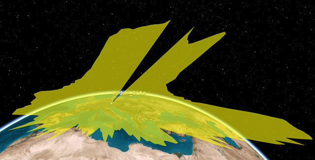
Sensor Field of View
Your image might look different from the image in this tutorial. You can orient the 3D Graphics window to obtain the same view, but it's not required.
If you were only using the Line of Sight constraint, the sensor's field of view would be circular. In this instance, you are taking into account the central body (Earth) and terrain, which is causing the blockage of the sensor's field of view.
Inserting the satellites
The radar site's primary purpose is to track three Technology Development satellites.
- Bring the Insert STK Objects tool () to the front.
- Insert a Satellite (
 ) object using the From Standard Object Database (
 ) method.
 - Set the following search criteria when the Search Standard Object Database dialog box opens:
- Click .
- Multi-select MAROC-TUBSAT, BeeSat and DLR-Tubsat in the Results list.
- Click .
- Click to exit the Standard Object Database tool after the satellites are propagated.
| Option | Value |
|---|---|
| Owner | Germany |
| Mission | Technology Development |
Determining benchmark access to the satellites
Determine the total time each satellite appears within the sensor's field of view. That is considered the total access duration. You will use this value as a benchmark to see if the radome affects accesses to the satellites.
Computing access
The STK application
- Right-click on Radar_FOV () in the Object Browser.
- Select Access... (
 ) in the shortcut menu.
 - Select all three Satellite () objects in the Associated Objects list when the Access tool opens.
- Click
 .
.
Generating an Access report
An
- Click in the Reports panel.
- Scroll to the bottom of the report.
- Note the value of the Total Duration in the Global Statistics section (for example, approximately 15,100 seconds).
Saving the Access report as an external text file
Save the Access report outside of the STK application. This is a safe way to retain the original analysis values.
- Return to the Access report.
- Click Save as text () in the Access report toolbar.
- Ensure your scenario folder displays in the in Address bar in the Save Report dialog box.
- Enter Sensor to Satellites Terrain Only in the File name field.
- Click .
- Close the Access report.
- Close the Access tool.
Modeling the communications radome
Construction crews plan to build a large communications site radome less than one-half kilometer from the proposed radar site. You want to model the radome to analyze potential interference.
Inserting another facility object
Use another Facility object as the radar site location.
- Bring the Insert STK Objects tool () to the front.
- Insert a Facility () object using the Insert Default () method.
- Rename Facility2 () Comm_Radome.
- Open Comm_Radome's () Properties ().
- Select the Basic - Position page.
- Set the following position options:
- Click to confirm your changes and to close the Properties Browser.
| Option | Value |
|---|---|
| Latitude | 47.899 deg |
| Longitude | 11.1113 deg |
Viewing the communications radome in relation to the radar field of view
View the radome in the 3D Graphics window.
- Bring the 3D Graphics window to the front.
- Right-click on Comm_Radome () in the Object Browser.
- Select Zoom To in the shortcut menu.
- Change your view so that you can see both the communications site radome and the and radar site.
- Use your mouse to set the view so that you can see how Radar_FOV's () projection cuts through Comm_Radome's () 3D Model.
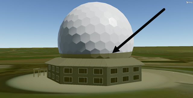
Sensor Field of View Passing Through 3D Graphics Model
If you look closely, you can see that the sensor's projection cuts through the communications site's radome. The Facility object's 3D Graphics model is not being used as an obstruction during analysis. In order to use it as an obscuring object, you must use the AzEl Mask tool.
In this scenario, you're using a Facility object to simulate the communications site's radome. If you were actually performing this analysis against an actual building, you would need to consider creating your own 3D model built to specifications.
Using the AzEl Mask tool
Use the AzEl Mask tool to create a body mask file (.bmsk) that can be used in access computations and visualization.
Opening the AzEl Mask tool
You can access the AzEl Mask tool from the Sensor menu in the Menu Bar.
- Maximize your 3D Graphics window.
- Select Radar_FOV () in the Object Browser.
- Select the Sensor menu in the Menu Bar at the top of the STK application.
- Select AzEl Mask... in the Sensor menu.
Preparing the AzEl Mask tool
Start by setting up the AzEl Mask tool prior to creating a body mask file. The tool's Az/El Mask View window allows you to see the obscuring objects in the six views used in generating the contours. The views will be shown in successive fashion when the Compute button is clicked. The tool's AzEl Mask dialog box enables you to identify obscuring objects and define the instant in time at which obscuration contours are computed. Set Comm_Radome as the obscuring object and the window dimension to 500.
- Move the AzEl Mask dialog box (AzElMask for Radar_FOV) to the right so that it isn't on top of the Az/El Mask View window.
- Select Comm_Radome () in the AzEl Mask window's Obscuring Objects list.
- Set the Window Dim value to 500 in the Data panel.
- Click .
- Click
- Ensure your .bmsk file is being saved in your scenario folder when the Select Body Mask File dialog box opens. Use the default file name.
- Click .
- Close the AzEl Mask dialog box and the Az/El Mask View window when the computation is complete.
The Obscuring Objects list contains the central bodies and scenario objects that are candidates for obscuring the sensor's field of view.
Larger window sizes produce more accurate masks which require more access computation time. A mask file cannot be generated if the window dimensions are too small or if they are larger than the STK workspace. If the Dim value of 500 places this window outside of your STK workspace, decrease the value until it's inside the STK workspace.
Constraining the sensor with the AzEl Mask
Use the body mask file as the
- Open Radar_FOV's () Properties ().
- Select the Basic - Sensor AzEl Mask page.
- Open the Use drop-down list.
- Select MaskFile.
- Click the Mask File ellipsis ().
- Browse to your scenario folder, if required, when the Select File dialog box opens.
- Select Radar_FOV.bmsk in the list.
- Click .
- Select the Use Mask for Access Constraint check box.
- Click to accept your changes and to keep the Properties Browser open.
Visualizing the sensor AzEl Mask
In order to visualize the Sensor AzEl Mask constraint, follow the same procedure as you did to visualize the terrain Az-El Mask.
- Select the 2D Graphics - Projection page.
- Leave AzElMask selected in the Field of View - Use Constraints panel.
- Scroll down the Field of View - Constraints list until you locate SensorAzElMask.
- Use Ctrl + click to select SensorAzElMask in the list in addition to AzElMask, which you selected earlier.
- Click to confirm your changes and to close the Properties Browser.
Viewing the sensor AzEl Mask in the 3D Graphics window
You can view the constrained FOV in the 3D Graphics window.
- Bring the 3D Graphics window to the front.
- Zoom To Radar_Site ().
- Change your view so that you can see Radar_Site (), Comm_Radome (), and Radar_FOV's () field of view being affected by Comm_Radome ().
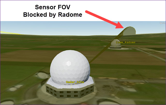
Sensor FOV Blocked by The Radome
Determining changes to the total access duration
Determine the total time each satellite appears within the sensor's field of view now that the sensor FOV takes obscuration by the radome into account using the Sensor AzEl mask.
- Right-click on Radar_FOV () in the Object Browser.
- Select Access... () in the shortcut menu.
- Select all three Satellite () objects in the Access tool's Associated Objects list.
- Click in the Reports panel.
- Scroll to the bottom of the report.
- Note the Total Duration value in the Global Statistics section (for example, approximately 15,000 seconds).
Comparing the access data
Compare access data between the total access durations when using just the AzEl mask and when using boht th terrain AzEl mask and the facility body mask file. The best result would be that you don't lose any of the total access duration.
- Open Windows File Explorer.
- Browse to your scenario folder (e.g. C:\Users\<username>\Documents\STK_ODTK 13\AzElMask_Volumetrics).
- Open the Sensor to Satellites Terrain Only.txt file.
- Return to the STK application.
- Compare the Global Statistics Total Duration time in the text file to the Total Duration time in the Access Report.
- Close both reports and the Access tool when finished.
Did the communications site radome affect your total duration access time?
Using Volumetric Analysis and the Analysis Workbench to analyze the radar's field of view
Based on the curvature of the Earth and that the satellites being tracked by the radar are in a low Earth orbit (LEO), you want to determine how much of the radar's field of view is blocked by the Earth itself, surrounding terrain, and the radome within a 3,000-kilometer radius from the radar site. In order to determine how much the radar field of view is affected, you will use an Area Target object in conjunction with the Volumetric Analysis capability and the Analysis Workbench capability's Time tool and Spatial Analysis tool to analyze a 3D volume of space inside the portion of a spherical sector between 10 and 700 kilometers in altitude from the radar site.
Inserting an Area Target object
Insert an Area Target (![]() ) object to model the 3,000-kilometer radius analysis area on the globe.
) object to model the 3,000-kilometer radius analysis area on the globe.
- Bring the Insert STK Objects tool () to the front.
- Insert an Area Target (
 ) object using the Area Target Wizard (
 ) method.
 - Set the following options in the Area Target Wizard ():
- Click to confirm your changes and to close the Area Target Wizard.
| Option | Value |
|---|---|
| Name | OpsArea |
| Area Type | Ellipse |
| Semi-Major Axis | 3000 km |
| Semi-Minor Axis | 3000 km |
| Centroid - Latitude | 47.8996 deg |
| Centroid - Longitude | 11.1142 deg |
Viewing the Area Target object in the 3D Graphics window
View the Area Target in the 3D Graphics window.
- Bring the 3D Graphics window to the front.
- Click Home View () in the 3D Graphics window toolbar.
- Move your view so that you can see OpsArea ().
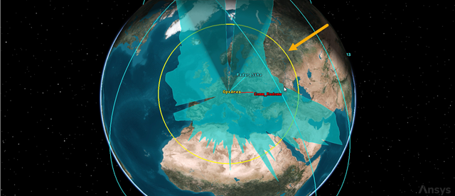
3D Graphics View of the Area Target
Opening the Time tool
There is no need to calculate the radar's field of view for the entire 24-hour analysis period. Use the Analysis Workbench capability's
- Right-click on AzElMask_Volumetrics () in the Object Browser.
- Select Analysis Workbench... (
 ) in the shortcut menu.
 - Select the Time tab when the Analysis Workbench opens.
- Ensure AzElMask_Volumetrics () is selected in the Object list on the left.
Creating a Fixed Interval
An Interval component produces a single interval of time. You want a to create a one-second Fixed Interval to use in your analysis.
- Click Create new Interval (
 ).
). - Click for Type when the Add Time Component dialog box opens.
- Select Fixed Interval () in the Select Component Type list when the Select Component Dialog box opens.
- Click to confirm your selection and to close the Select Component Dialog box.
- Enter One_Second in the Name field.
- Enter 15 Mar 2024 12:00:01.000 UTCG in the Stop Time field.
- Click to confirm your changes and to close the Add Time Component dialog box.
Creating a Cartographic Volume grid
Use the Spatial Analysis tool create two
- Select the Spatial Analysis tab at the top of the Analysis Workbench.
- Select OpsArea () in the object list.
- Click Create new Volume Grid (
 ).
). - Ensure the Type is Cartographic in the Add Spatial Analysis Component dialog box.
- Enter Ref_Grid in the Name field.
- Look at the following check boxes:
- Automatically fit to Area Target: when selected, this attaches the center of the grid to the Area Target's centroid.
- Constrain active grid points within Area Target: when selected, this tells the STK software to analyze the grid points contained inside the Area Target, not the overflow points outside the Area Target.
- Click
- Set the following values in the Altitude panel when the Grid Values dialog box opens:
- Click to close the Grid Values dialog box.
- Click to close the Add Spatial Analysis Component dialog box.
A Cartographic grid uses latitude, longitude and altitude based on a central body reference ellipsoid.
| Option | Value |
|---|---|
| Minimum | 10 km |
| Maximum | 700 km |
| Number of Steps | 20 |
The number of steps determines how many grid points are added to the volume for computation and analysis.
Creating a Constrained Volume grid
A Constrained Volume grid is one in which the grid points from the reference grid are available only when a specified
- Select OpsArea () in the Object list.
- Click Create New Volume Grid ().
- Enter OpsArea_Constrained in the Name field when the Add Spatial Analysis Component dialog box opens.
- Click for Type.
- Select Constrained () in the Select Component Type list when the Select Component Type dialog box opens.
- Click to confirm your selection and to close the Select Component Type dialog box.
Selecting the Reference grid
Select the Cartographic grid you created previously as the Reference grid.
- Click the Reference Grid ellipsis ().
- Select OpsArea () in the Object list when the Select Reference Volume Grid dialog box opens.
- Select Ref_Grid () in the Volume Grids for: OpsArea list.
- Click to close the Select Reference Volume Grid dialog box.
Choosing the spatial condition
Select the Radar_FOV's (![]() ) Visibility as the spatial condition used for the volumetric analysis.
) Visibility as the spatial condition used for the volumetric analysis.
- Click the Spatial Condition ellipsis () when you return to the Select Reference Spatial Condition dialog box.
- Select Radar_FOV () in the object list when the Select Reference Spatial Condition dialog box opens.
- Select Visibility (
 ) in the Spatial Conditions for: Radar_FOV list.
 - Click to close the Select Reference Spatial Condition dialog box.
- Click to close the Add Spatial Analysis Component dialog box.
- Click to close the Analysis Workbench.
This will apply the constrained visibility of Radar_FOV (![]() ) to the 3D Volume grid.
) to the 3D Volume grid.
Inserting a Volumetric object
Insert a new Volumetric object into your scenario.
- Bring the Insert STK Objects tool () to the front.
- Insert a Volumetric (
 ) object using the Insert Default () method.
Defining the Volume Grid
The default Volume grid encircles the Earth up to an altitude of 1,000 kilometers. Change the grid's
- Open the Volumetric1's () Properties ().
- Select the Basic - Definition page.
- Click the Volume Grid ellipsis ().
- Select OpsArea () in the Object list when the Select Volume Grid for Volumetric1 dialog box opens.
- Select OpsArea_Constrained () in the Volume Grids for: OpsArea list.
- Click to close the Select Volume Grid for Volumetric1 dialog box.
- Click to accept your changes and to keep the Properties Browser open.
Selecting the Spatial Calculation
A Spatial Calculation is a scalar calculation that depends on both time and location.
- Select the Spatial Calculation check box.
- Click the Spatial Calculation ellipsis ().
- Select OpsArea () in the Object list when the Select Spatial Calculation for Volumetric1 dialog box opens.
- Select Altitude (
 ) in the Spatial Calculations for: OpsArea list.
 - Click to close the Select Spatial Calculation for Volumetric1 dialog box.
- Click to accept your changes and to keep the Properties Browser open.
Selecting the analysis Interval
To evaluate the Spatial Calculation on your Volume grid, update the Volumetric object's
- Select the Basic - Interval page.
- Click the Analysis Interval ellipsis ().
- Select AzElMask_Volumetrics () in the object list when the Select Interval or List dialog box opens.
- Select One_Second () in the Components for: AzElMask_Volumetrics list.
- Click to close the Select Interval or List dialog box.
- Click to accept your selection and to keep the Properties Browser open.
- Save () your scenario.
Computing visibility inside the grid
With your analysis configured,
- Select Volumetric1 () in the Object Browser.
- Select the Volumetric menu in the Menu Bar.
- Select Compute.
Generating a Satisfaction Volume report
Generate a report that shows how much of the radar's field of view is visible. The
- Right-click on Volumetric1 () in the Object Browser.
- Select Report & Graph Manager... (
 ) in the shortcut menu.
 - Select the Satisfaction Volume (
 ) report in the Installed Styles (
 ) folder when the Report & Graph Manager opens.
 - Click .
- Close the Satisfaction Volume report and the Report & Graph Manager when finished.
You can see in the report that the radar field is approximately 44 percent satisfied. Remember, you computed this starting at a low altitude of only 10 kilometers; there will be more losses at lower altitudes due to the central body (Earth), terrain and the radome.
Displaying visibility inside the grid
The Volumetric object's
- Return to Volumetric1's () Properties.
- Select the 3D Graphics - Grid page.
- Clear the Show Grid check box.
- Click .
This will make the grid look better for a briefing or presentation. If you were analyzing something like Bit Error Rates per grid point, you might leave this on. By clicking on a point in the 3D Graphics window, you will receive a value for that point. In this scenario, they are on or off.
Adding Spatial Calculation levels
Update the Volumetric object's
- Select the 3D Graphics - Volume page.
- Select the Spatial Calculation Levels option.
- Click at the bottom of the page.
- Set the following when the Insert Evenly Spaced Values dialog box opens:
- Click .
| Option | Value |
|---|---|
| Units | km |
| Start Value | 10 |
| Stop Value | 700 |
| Step Size | 100 |
Adjusting the translucency
You can adjust translucency of the colors in order to make the levels stick out or fade depending on your desired view. In this case, you want to be able to see the lower altitude colors more than the higher altitude colors. The Earth, terrain, and the communications radome affect the lower-altitude colors more than the higher altitude colors. You can use the Translucency slider or manually type in the percentage. In this case, type them in.
- Set the following in the % column, which is located in the Fill Levels list:
- Click .
| Value km | % |
|---|---|
| 10 | 10 |
| 110 | 20 |
| 210 | 40 |
| 310 | 40 |
| 410 | 50 |
| 510 | 50 |
| 610 | 60 |
| 700 | 60 |
Displaying a 3D Graphics Legend
The Volumetric object's
- Select the 3D Graphics - Legends page.
- Select the Fill Legend tab.
- Set the following options:
- Click .
| Option | Value |
|---|---|
| Show Legend | Selected |
| Text Options - Title | Altitude (km) |
| Text Options - Number Of Decimal Digits | 0 |
| Range Color Options - Color Square Width (pixels) | 40 |
Viewing the Volumetric contours
- Bring the 3D Graphics window to the front.
- Use your mouse to change your view to get an idea of how obscurations affect the different levels of altitude.
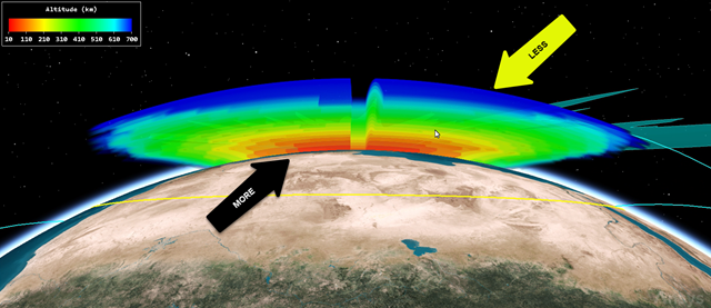
Radar Field of View Obscuration
Summary
You loaded analytical terrain into your scenario that covers the area in which the radar site is going to be built. You then used a Sensor object to create the field of view of the radar. You propagated two satellites and generated an access between the sensor and the satellites to create a benchmark access time. Next, you placed a Facility object where a new communications radome will be constructed. You used the AzEl Mask tool to determine if the radome affects the sensor's field of view. Generating another Access report, you determined that the radome will affect your overall access time to the satellites. Next, you used the Analysis Workbench Time tool to create a one second interval to be used with a Volumetric object's compute time. Then, using the Analysis Workbench Spatial Analysis tool, you created a reference grid inside of an Area Target object and a constrained grid which then applied the Sensor object's constraints to the 3D volume of space. You determined that a significant amount of your volume is obscured by the Earth, terrain and the radome.
On your own
Throughout the tutorial, hyperlinks were provided that pointed to in depth information of various tools and functions. Now's a good time to go back through this tutorial and view that information. You can add other models to your scenario and determine their obscuration affects. You can adjust the altitude of your reference grid and recalculate volume obscuration. Have fun!