Part 8:
STK Pro, STK Premium (Air), STK Premium (Space), or STK Enterprise
You can obtain the necessary licenses for this tutorial by contacting AGI Support at support@agi.com or 1-800-924-7244.
The results of the tutorial may vary depending on the user settings and data enabled (online operations, terrain server, dynamic Earth data, etc.). It is acceptable to have different results.
This lesson requires STK 12.9 or newer to complete.
Capabilities covered
This lesson covers the following STK Capabilities:
- STK Pro
- Coverage
Problem statement
Engineers and operators need to analyze global or regional coverage from one asset or from a collection of assets. They might need to account for constraints such as sunlight and terrain. They may need to simply analyze if a sensor footprint passes over a specific ground location, or they may need to analyze a large area of ground or space and determine communication bit error rates in terms of area of interest, age of data, dilution of precision, etc. In this lesson, you will analyze three satellites and their sensor footprints on the Earth's surface. You need to determine what percentage of the Earth's surface is seen by all three sensors during a 24-hour period while taking into consideration sunlight, umbra, and how many times points on the ground are accessed. Then, you need to determine how long one satellite sensor covers Canada and the continental United States during the same 24-hour period.
Solution
Use STK to model Earth-observing payloads attached to sensors located in three different orbits. Use STK's Coverage capability to model and analyze the quality and quantity of coverage provided by the three payloads to determine the following:
- The percentage of the Earth's surface the satellite payloads survey during a 24-hour period and daylight hours only
- How many times the satellite payloads survey points on the ground during a 24-hour period and daylight hours only
- How long points on the ground are seen in Canada and the continental United States
What you will learn
Upon completion of this tutorial, you will be able to:
- Compute global coverage
- Compute coverage in designated areas
- Understand a coverage grid
- Use constraints in a coverage grid
- Determine coverage assets
- Choose which data providers supply answers to your questions
- Create color contours pertaining to the coverage analysis in the 2D and 3D Graphics windows
Video guidance
Watch the following video. Then follow the steps below, which incorporate the systems and missions you work on (sample inputs provided).
Create a new scenario
Create a new scenario.
- Launch STK (
 ).
). - Click Create a Scenario (
 ) in the Welcome to STK window.
 - Enter the following in the STK: New Scenario Wizard:
- Click when you finish.
- Click Save (
 ) when the scenario loads. A folder with the same name as your scenario is created for you in the location specified above.
 - Verify the scenario name and location in the Save As dialog box.
- Click .
| Option | Value |
|---|---|
| Name | STK_Coverage |
| Location | Default |
| Start | 15 Mar 2024 16:00:00.000 UTCG |
| Stop | 16 Mar 2024 16:00:00.000 UTCG |
Save (![]() ) often!
) often!
Viewing both the 2D and 3D Graphics windows
You can view coverage in both the 2D and 3D Graphics windows. Placing them side by side makes this simple to do.
- Close (
 ) the Timeline View at the bottom of STK.
 - Extend the Window menu.
- Select Tile Vertically to evenly space the windows side-by-side in the integrated workspace.
Turning off Terrain Server
Analytical and visual terrain is not required in this analysis. Turn off the Terrain Server.
- Right-click STK_Coverage () in the Object Browser.
- Select Properties (
 ).
). - Select the Basic - Terrain page when the Properties Browser opens.
- Clear the Use terrain server for analysis check box.
- Click to accept your changes and to close the Properties Browser.
Creating a satellite in a circular orbit
Insert the first Satellite (![]() ) and place it in a circular orbit. Circular orbits have a constant radius.
) and place it in a circular orbit. Circular orbits have a constant radius.
- Select Satellite (
 ) in the Insert STK Objects tool.
 - Select the Orbit Wizard (
 ) method.
 - Click .
- Set the following in the Orbit Wizard:
- Click to propagate the Satellite () object using the default J4Perturbation propagator and to close the Orbit Wizard.
| Option | Value |
|---|---|
| Type | Circular |
| Satellite Name | Circ_Sat |
| Inclination | 55 deg |
| Altitude | 700 km |
| RAAN: | -105 deg |
Creating a satellite in a repeating ground trace orbit
Insert the second Satellite (![]() ) and place it in a repeating ground trace orbit. Orbits with repeating ground traces are useful when you want identical viewing conditions at different times to detect changes. You can have the ground trace repeat every day or interweave from day to day before repeating.
) and place it in a repeating ground trace orbit. Orbits with repeating ground traces are useful when you want identical viewing conditions at different times to detect changes. You can have the ground trace repeat every day or interweave from day to day before repeating.
- Insert a Satellite () object using the Orbit Wizard () method.
- Set the following in the Orbit Wizard:
- Click .
| Option | Value |
|---|---|
| Type | Repeating Ground Trace |
| Satellite Name | Repeat_Sat |
Creating a satellite in a sun-synchronous orbit
Insert the third Satellite (![]() ) and place it in a sun-synchronous orbit. These orbits are designed to utilize the effect of the Earth's oblateness, causing the orbit plane to precess at a rate equal to the mean orbital rate of the Earth around the Sun. Sun synchronous orbits have the property that their nodes maintain constant local mean solar times.
) and place it in a sun-synchronous orbit. These orbits are designed to utilize the effect of the Earth's oblateness, causing the orbit plane to precess at a rate equal to the mean orbital rate of the Earth around the Sun. Sun synchronous orbits have the property that their nodes maintain constant local mean solar times.
- Insert a Satellite () object using the Orbit Wizard () method.
- Set the following in the Orbit Wizard:
- Click .
| Option | Value |
|---|---|
| Type | Sun Synchronous |
| Satellite Name | Sun_Sat |
Adding payloads
All three satellites use the same sensor type and size. STK enables you to copy and paste objects from one object to another. You will set up the first sensor and then copy and paste it to the other two. All you'll have to do is rename them or STK will use the same name with a one-up number.
Inserting a Sensor object
Attach a Sensor (![]() ) object to Circ_Sat (
) object to Circ_Sat (![]() ). Define a rectangular sensor with a 20-degree vertical half-angle and 10-degree horizontal half-angle.
). Define a rectangular sensor with a 20-degree vertical half-angle and 10-degree horizontal half-angle.
- Insert a Sensor (
 ) object using the Define Properties () method.
 - Select Circ_Sat () in the Select Object dialog box.
- Click .
- Select the Basic - Definition page when the Properties Browser opens.
- Set the following:
- Click to accept your changes and to close the Properties Browser.
| Option | Value |
|---|---|
| Sensor Type | Rectangular |
| Vertical Half Angle | 20 deg |
| Horizontal Half Angle | 10 deg |
Reusing the Sensor object
Copy and paste the rectangular sensor onto the other two satellites.
- Select Sensor1 (
 ) in the Object Browser .
 - Click Copy (
 ) in the Object Browser toolbar.
 - Select Repeat_Sat (
 ) in the Object Browser.
 - Click Paste (
 ) in the Object Browser toolbar.
 - Select Sun_Sat () in the Object Browser.
- Click Paste () in the Object Browser toolbar.
Renaming the Sensor Objects
Rename the three sensors.
- Right-click on Sensor1 (
 ) in the Object Browser.
 - Select Rename in the shortcut menu.
- Rename Sensor1 () to Circ_Sens.
- Press Enter on your keyboard.
- Repeat the steps above to rename Sensor2 () to Repeat_Sens and Sensor3 () to Sun_Sens.
Adding a Coverage Definition object
The Coverage Definition object defines a coverage area for analysis.
Inserting a Coverage Definition object
Insert a Coverage Definition (![]() ) object into your scenario.
) object into your scenario.
- Insert a Coverage Definition (
 ) object using the Insert Default () method.
 - Rename CoverageDefinition1 () to World_Cov.
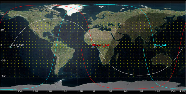
2D Graphics Window Default Coverage Grid
The grid area of interest default setting is latitude bounds and covers 60 degrees south latitude to 70 degrees north latitude. The point granularity defaults to every 6 degrees and sits on the surface of the WGS84. You can determine the spacing between grid points using grid definition options. These options help you define the fineness or coarseness of the grid. The use of finer grid resolutions typically produce more accurate results, but requires additional computational time and resources.
Defining the coverage grid
Define the coverage grid to be global, with a 4-degree point granularity.
- Open World_Cov's () Properties ().
- Select the Basic - Grid page when the Properties Browser opens.
- Open the Type: shortcut menu in the Grid Area of Interest panel.
- Select Global.
- Enter 4 deg in the Lat/Lon field located in the Point Granularity panel.
- Click to accept your changes and to keep the Properties Browser open.
- Select the 3D Graphics window to bring it to the front. Notice the grid covers the entire globe and the grid spacing is 4 degrees.
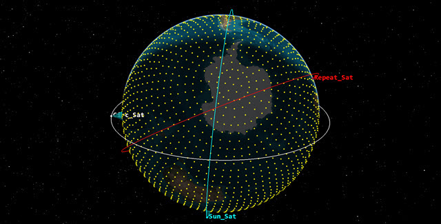
3D Graphics Window Global Coverage Grid
Assigning coverage assets
Assets properties allow you to specify the STK objects used to provide coverage. Define the three sensors as the Coverage Assets.
- Return to World_Cov's () properties ().
- Select the Basic - Assets page.
- Expand (
 ) Circ_Sat (), Repeat_Sat () and Sun_Sat () in the Assets list.
 - Select Circ_Sens (), Repeat_Sens () and Sun_Sens ().
- Click .
- Click to accept your changes and to keep the Properties Browser open.
Turning off automatic recomputation of accesses
STK automatically recomputes accesses every time you update an object on which the coverage definition depends (such as an asset). If you want control as to when STK computes coverage, you need to turn this off.
- Select the Basic - Advanced page.
- Clear the Automatically Recompute Accesses check box.
- Click to accept your changes and to close the Properties Browser.
Using the Compute Accesses tool
The ultimate goal of coverage is to analyze accesses to an area by using assigned assets and applying necessary limitations upon those accesses. Compute coverage with the Compute Accesses tool.
- Select World_Cov () in the Object Browser.
- Extend the CoverageDefinition menu.
- Select Compute Accesses.
You can view the progress bar in the lower-right corner of STK.
Generating a coverage by latitude graph
A coverage by latitude graph uses the Coverage by Latitude data provider. This analyzes coverage for each latitude in the selected range at intervals depending on the selected resolution. It uses the Latitude and Percent Time Covered elements.
- Right-click on World_Cov () in the Object Browser.
- Select Report & Graph Manager... (
 ) in the shortcut menu.
 - Select the Coverage By Latitude graph (
 ) in the Installed Styles list.
 - Click .
- Close () the graph.
- Click to close the Report & Graph Manager.
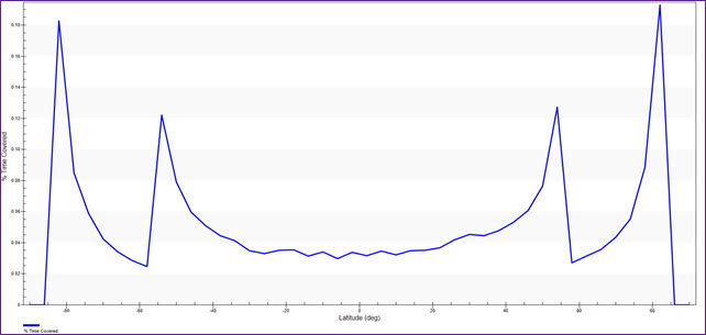
Coverage By Latitude Graph
The Coverage By Latitude graph is a quick way to see the percentage of time covered by latitude.
Figure of Merit
STK enables you to specify the method by which the quality of coverage is measured using a Figure Of Merit (![]() ) object.
) object.
Inserting a Figure of Merit
Insert a Figure of Merit object.
- Insert a Figure Of Merit (
 ) object using the Insert Default () method.
 - Select World_Cov (
 ) in the Select Object dialog box.
 - Click .
- Rename FigureOfMerit1 () to Simple_Cov.
Measuring Simple Coverage
Simple Coverage measures whether or not a point is accessible by any of the assigned assets during the analysis period. Areas on the map that are shaded mean that the surface point is seen by at least one sensor footprint during the 24-hour analysis period.
- Open Simple_Cov's () Properties ().
- Select the Basic - Definition page when the Properties Browser opens.
- Look at the Definition - Type. It defaults to Simple Coverage.
- Click to close the Properties Browser without making any changes.
- Bring the 2D Graphics window to the front.
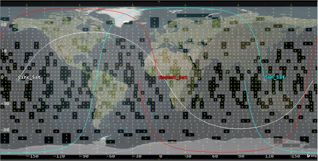
Simple Coverage Graphics
Your 2D Graphics window may display different colors than the image above. You can change the color in Simple_Cov's (![]() ) 2D Graphics - Static properties page.
) 2D Graphics - Static properties page.
Reporting Percent Satisfied
Generate a Percent Satisfied report. This presents the percentage of the total grid area where the static value of the Figure Of Merit meets the specified satisfaction criterion. In this scenario, the report shows the percentage of the globe that is accessible by any of the three sensors during the analysis period.
- Right-click Simple_Cov () in the Object Browser.
- Select Report & Graph Manager... () in the shortcut menu.
- Select the Percent Satisfied report (
 ) in the Installed Styles list.
 - Click .
- Note the % Satisfied value at the bottom of the report (e.g., ~77%).
- Close the report and the Report & Graph Manager when finished.
Approximately 77% of the globe is covered by at least one of the three sensors during the analysis time period.
Creating a constraint
Once you have defined the grid area, you can specify an object class or a specific object for the points within the grid. You are interested in the percentage of coverage during periods of direct sun.
Creating a Target object
Insert a Target (![]() ) object and define a direct sun lighting constraint.
) object and define a direct sun lighting constraint.
- Insert a Target (
 ) object using the Define Properties () method.
 - Select the Constraints - Active page when the Properties Browser opens.
- Click Add new constraints (
 ) in the Active Constraints toolbar.
 - Type Lighting in the Search: field when the Select Constraints to Add dialog box opens.
- Select Lighting in the Constraint Name list.
- Click .
- Click to close the Select Constraints to Add dialog box.
- Look at the Lighting Constraint Name. DirectSun is the default Value.
- Click to accept your changes and to close the Properties Browser.
- Rename Target1 () to Constraint_Template.
- Clear the check box next to Constraint_Template (
 ) in the Object Browser. There is no need to see Constraint_Template () on the 2D or 3D Graphics windows.
Applying the grid constraint
Set the Constraint_Template (![]() ) as the grid constraint.
) as the grid constraint.
- Open World_Cov's (
 ) Properties ().
 - Select the Basic - Grid page when the Properties Browser opens.
- Click in the Grid Definition panel.
- You can see that the Reference Constraint Class defaults to Target in the Grid Constraint Options dialog box.
- Select the Use Object Instance check box.
- Select Constraint_Template in the list.
- Click to close the Grid Constraints Options dialog box.
- Click to accept your changes and to close the Properties Browser.
For all object classes, the Basic properties of the object, excluding positional information, are applied to the grid points.
Recomputing accesses
Since a change was made to the coverage grid, you need to recompute accesses.
- Select World_Cov () in the Object Browser.
- Extend the CoverageDefinition menu.
- Select Compute Accesses.
- Bring the 2D Graphics window to the front when finished.
Determining Coverage Loss
It's obvious from the view in the 2D Graphics window that you have less coverage using a Direct Sun constraint. Due to the analysis time period, there is more sunlight in the northern hemisphere that you can see on the map. Generate a Percent Satisfied report to determine the percent coverage loss.

Simple Coverage with Direct Sun Constraint
- Right-click Simple_Cov () in the Object Browser.
- Select Report & Graph Manager... () in the shortcut menu.
- Select the Percent Satisfied report () in My Favorites
- Click .
- Note the % Satisfied value at the bottom of the report (e.g., ~51 %).
- Close report and the Report & Graph Manager when finished.
Since coverage is now being analyzed during periods of direct sun and not being analyzed during periods of umbra, there's a significant loss of coverage.
Measuring Number of Accesses
Insert a new Figure of Merit to measure Number of Accesses. This will measure the number of independent accesses of points.
- Clear the check box next to Simple_Cov () in the Object Browser.
- Insert a Figure Of Merit () object using the Define Properties () method.
- Select World_Cov () in the Select Object dialog box.
- Click .
- Select the Basic - Definition page when the Properties Browser opens.
- Open the Type: shortcut menu in the Definition panel.
- Select Number Of Accesses.
- Keep Compute set to the default Total.
- Click to accept your changes and to close the Properties Browser.
- Rename FigureOfMerit2 () to Num_Access.
Total computes the total number of accesses over the coverage interval without considering overlapping accesses.
Generating a Grid Stats report
Generate a Grid Stats report to see the smallest to largest number of accesses to any point in the grid.
- Right-click Num_Access () in the Object Browser.
- Select Report & Graph Manager... () in the shortcut menu.
- Select the Grid Stats report () in the Installed Styles list.
- Click .
- Note the Maximum value (e.g., 6).
- Note the Minimum value (e.g., 0).
- Close the report and the Report & Graph Manager when finished.
- Clear the check box next to World_Cov () in the Object Browser.
That means at least one point in the grid was accessed on six (6) different occasions during the analysis period.
That means at least one point in the grid was never accessed by any of the three sensors during the analysis period.
Creating an Area Target object for coverage
You can focus the coverage grid in a confined location using Area Target (![]() ) objects. For this part of the analysis, you will focus on the continental United States and mainland Canada. You will ignore islands and territories.
) objects. For this part of the analysis, you will focus on the continental United States and mainland Canada. You will ignore islands and territories.
Insert an Area Target (![]() ) to model Canada and the Continental United States.
) to model Canada and the Continental United States.
- Insert an Area Target (
 ) object using the Select Countries and US States (
 ) method.
 - Clear the US States check box in the List Selections panel when the Select Countries And US States dialog box opens.
- Use the Ctrl key to select Canada and United_States_of_America in the countries list on the left. You can insert them individually if desired.
- Click .
- Click to close the Select Countries And US States dialog box.
Defining a new Coverage Definition
You want to determine coverage time inside the boundaries of the Area Target (![]() ) objects. You will use Repeat_Sens (
) objects. You will use Repeat_Sens (![]() ) as the asset. No constraints are necessary.
) as the asset. No constraints are necessary.
Inserting a Coverage Definition
Insert a new Coverage Definition (![]() ).
).
- Insert a Coverage Definition () object using the Insert Default () method.
- Rename CoverageDefinition2 () to Country_Cov.
Define Coverage Grid
Define the coverage area of interest to be Canada and the continental United States using the Area Targets (![]() ).
).
- Open Country_Cov's () properties ().
- Select the Basic - Grid page when the Properties Browser opens.
- Open the Type: shortcut menu in the Grid Area of Interest panel.
- Select Custom Regions.
- Open the next shortcut menu below Type:.
- Select Area Targets.
- Use the Ctrl key to select Canda and United_States_of_America in the Area Targets list on the left.
- Move (
 ) Canada () and United_States_of_America () from the Area Targets list to the Selected Regions list.
 - Enter 1 deg in the Lat/Lon field located in the Point Granularity field.
- Click to accept your changes and to keep the Properties Browser open.
- Bring the 2D Graphics window to the front.
- Zoom In (
 ) so that you only see Canada and United States.
 - If desired, you can Zoom In () and center the 3D Graphics window to the same view as the 2D Graphics window.

Coverage Grid Confined to Area Targets
Your 2D Graphics window may display different colors than the image above. The grid point colors can be changed by changing Country_Cov's (![]() ) color in the Object Browser or on Country_Cov's (
) color in the Object Browser or on Country_Cov's (![]() ) 2D Graphics - Attribute properties page.
) 2D Graphics - Attribute properties page.
Assigning a coverage asset
Define Repeat_Sens (![]() ) as the Coverage Asset.
) as the Coverage Asset.
- Return to Country_Cov's (
 ) properties ().
 - Select the Basic - Assets page.
- Expand () Repeat_Sat () in the Assets list.
- Select Repeat_Sens () in the Assets list.
- Click .
- Click to accept your changes and to keep the Properties Browser open.
Turning off grid display
You will display Figure Of Merit graphics, so turn off the grid point display.
- Select the 2D Graphics - Attributes page.
- Clear the Show Points check box in the Grid panel.
- Click to accept your changes and to close the Properties Browser.
This turns off the visual grid inside the Area Target (![]() ) object. Analytically, they're still there.
) object. Analytically, they're still there.
Computing accesses
You can compute accesses from the Object Browser vice the CoverageDefinition menu.
- Right-click Country_Cov () in the Object Browser.
- Select CoverageDefinition in the shortcut menu.
- Select Compute Accesses in the next shortcut menu.
Defining a Figure Of Merit object
Use a Figure Of Merit (![]() ) object to determine the amount of time during which the grid points are covered by Repeat_Sens (
) object to determine the amount of time during which the grid points are covered by Repeat_Sens (![]() ).
).
Inserting a Figure of Merit
Insert a Figure Of Merit (![]() ) to measure the quality of coverage of Country_Cov (
) to measure the quality of coverage of Country_Cov (![]() ).
).
- Insert a Figure Of Merit () object using the Insert Default () method.
- Select Country_Cov () in the Select Object dialog box.
- Click .
- Rename the FigureOfMerit3 (
 ) to Cov_Time.
Measuring Coverage Time
Set the Figure Of Merit to Coverage Time. It will measure the amount of time during which grid points are covered.
- Open Cov_Time's () properties ().
- Select the Basic - Definition page when the Properties Browser opens.
- Open the Type: shortcut menu in the Definition panel.
- Select Coverage Time.
- Open the Compute: shortcut menu.
- Select Total.
- Click to accept your changes and to keep the Properties Browser open.
Generating a Grid Stats report
Generate a report to determine the minimum and maximum amount of time any of the grid points are covered by Repeat_Sens (![]() ).
).
- Right-click Cov_Time () in the Object Browser.
- Select Report & Graph Manager... () in the shortcut menu.
- Select Grid Stats report () in the My Favorites list.
- Click .
- Note the Maximum (sec) (e.g., ~49 seconds).
- Return to Cov_Time's () properties ().
That means at least one point in the grid was accessed for a total of 49 seconds during the analysis period.
Defining static graphics for the Figure Of Merit
Define static graphics for the Figure Of Merit on the 2D Graphics - Static page.
- Select the 2D Graphics - Static page.
- Enter 30 in the % Translucency: field in the Show Points As panel.
- Select the Show Contours option in the Display Metric panel.
- Click in the Level Attributes panel.
- Set the following in the Level Adding panel:
- Click .
- Open the Start Color: shortcut menu in the Level Attributes panel.
- Select red.
- Open the End Color: shortcut menu
- Select blue.
- Select the Natural Neighbor option in the Contour Interpolation (points must be filled) panel.
- Click to accept your changes and to keep the Properties Browser open.
| Option | Value |
|---|---|
| Start | 0 sec |
| Stop | round down to the nearest integer from the Maximum (sec) value in the Grid Stats report (e.g. 49 sec) |
| Step | 5 sec |
Points with no coverage will be red and any points at or above your highest Level Attribute value will be blue.
Color is applied smoothly over all points in the grid to differentiate contour levels.
Set 2D and 3D Graphics windows legends
Once you have set the contours for coverage, you can set the display of the contour key, or legend.
- Click in the Level Attributes panel.
- Click to close Cov_Time's () properties ().
- Click in the Static Legend for Cov_Time dialog box.
- Set the following on the Figure of Merit Legend Layout dialog box:
- Click to close the Figure of Merit Legend Layout dialog box.
- Close () the Static Legend for Cov_Time dialog box.
- Bring the 2D and 3D Graphics windows to the front.
- Note Snap Frame (
 ) in both the 2D and 3D Graphics windows. You could use Snap Frame to take a picture of the map to place in a PowerPoint slide or in a document.
| Option | Value |
|---|---|
| 2D Graphics Window - Show at Pixel Location | on |
| 3D Graphics Window - Show at Pixel Location | on |
| Text Options - Title: | Coverage Time (seconds) |
| Text Options - Number Of Decimal Digits: | 0 |
| Range Color Options - Color Square Width (pixels): | 50 |
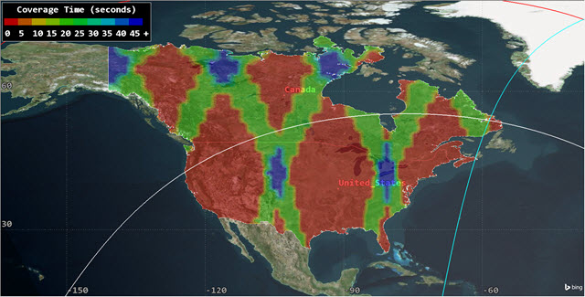
2D Graphics Window with Coverage Contours
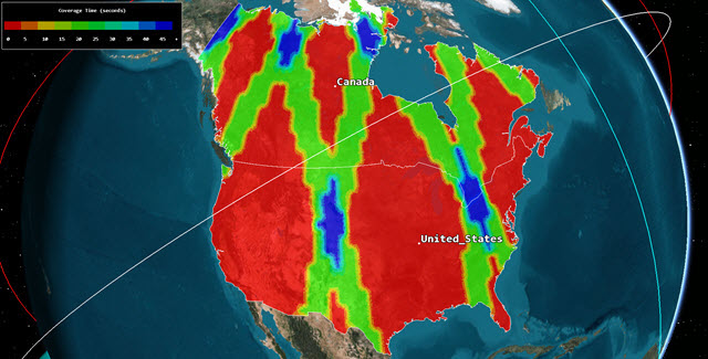
3D Graphics Window with Coverage Contours
Save your work
- Close any open reports, properties and the Report & Graph Manager.
- Save () your work.
Summary
You placed three Satellite (![]() ) objects into the scenario using circular, repeating ground trace and sun-synchronous orbits. All three satellites had similar Sensor (
) objects into the scenario using circular, repeating ground trace and sun-synchronous orbits. All three satellites had similar Sensor (![]() ) objects. You built a Coverage Definition (
) objects. You built a Coverage Definition (![]() ) object and set the grid definition to global. Using all three Sensor (
) object and set the grid definition to global. Using all three Sensor (![]() ) objects, you computed access. Using a Figure Of Merit (
) objects, you computed access. Using a Figure Of Merit (![]() ) object, you learned about Simple Coverage and how to analyze the percentage of the Earth accessed during a twenty four hour period. Next, you loaded a Target (
) object, you learned about Simple Coverage and how to analyze the percentage of the Earth accessed during a twenty four hour period. Next, you loaded a Target (![]() ) object at the Prime Meridian (default location), and set a direct sun constraint. Returning to the Coverage Definition (
) object at the Prime Meridian (default location), and set a direct sun constraint. Returning to the Coverage Definition (![]() ) object, you applied the constraint across the coverage grid and recalculated coverage to see how the direct sun constraint affected the percentage of coverage. The next step was to add a second Figure Of Merit (
) object, you applied the constraint across the coverage grid and recalculated coverage to see how the direct sun constraint affected the percentage of coverage. The next step was to add a second Figure Of Merit (![]() ) object and determine the number of accesses against each point in the coverage grid. Switching gears, you loaded two Area Target (
) object and determine the number of accesses against each point in the coverage grid. Switching gears, you loaded two Area Target (![]() ) objects which outlined the continental United States and Canada. With a new Coverage Definition (
) objects which outlined the continental United States and Canada. With a new Coverage Definition (![]() ) object, you focused coverage inside of the Area Target (
) object, you focused coverage inside of the Area Target (![]() ) objects using only the Sensor (
) objects using only the Sensor (![]() ) object attached to the satellite in the repeating ground trace orbit. This time, you configured a new Figure Of Merit (
) object attached to the satellite in the repeating ground trace orbit. This time, you configured a new Figure Of Merit (![]() ) object to focus on how long each point in the coverage grid was covered by the Sensor (
) object to focus on how long each point in the coverage grid was covered by the Sensor (![]() ) object. Finally, you learned how to apply static contours to both the 2D and 3D Graphics windows.
) object. Finally, you learned how to apply static contours to both the 2D and 3D Graphics windows.
On your own
Throughout the tutorial, hyperlinks are available that point o in-depth information of various subjects. Now's a good time to go back through this tutorial and view that information.
The following tutorials are recommended for further training:
-
Using STK Coverage teaches you animation contours.
-
Attitude Coverage combines features of STK Attitude and STK Coverage capabilities to enable you to analyze coverage in various directions over time, using several attitude-dependent figures of merit.
-
Getting started with STK Coverage focuses on setting up contours and how to analyze multiple sensors passing over a single point.
-
Modeling GPS Position Accuracy using STK Coverage covers navigation accuracy over the continental United States and how to calculate coverage against a single object.
-
Position Accuracy in Mountainous Terrain requires STK 12 or newer. It focuses on navigation accuracy in mountainous terrain and how terrain affects your coverage.