STK Pro, STK Premium (Air), STK Premium (Space), or STK Enterprise
You can obtain the necessary licenses for this tutorial by contacting AGI Support at support@agi.com or 1-800-924-7244.
This tutorial requires an internet connection and version 12.9 of the STK software or newer to complete in its entirety. If you have an earlier version of the STK software, you can view a legacy version of this lesson.
The results of the tutorial may vary depending on the user settings and data enabled (online operations, terrain server, dynamic Earth data, etc.). It is acceptable to have different results.
Capabilities covered
This lesson covers the following capabilities of the Ansys Systems Tool Kit® (STK®) digital mission engineering software:
- STK Pro
- Communications
Problem statement
Engineers and operators need to quickly determine communication link budgets. Factors such as communications unobstructed or obstructed by terrain, trees or man made structures need to be taken into consideration. Other factors that need to be included and analyzed are rain models, atmospheric losses, and RF interference sources. In this scenario, a team of scientists is monitoring glacial meltwater in a remote, mountainous location. Prior to setting up camp, they need to determine how their location will impact a link budget between them and a low earth orbit (LEO), Earth observation satellite, which is downloading data to the team.
Solution
Use STK Pro and the Communications capability to model and analyze a link budget between the ground site and the Earth observation satellite. The satellite transmitter will be analyzed using an isotropic, omnidirectional antenna pattern. The ground team will employ a small parabolic antenna steered by a servo motor that can track the satellite. After establishing a link budget based on line of sight only, terrain obstruction, rain, atmospheric absorption and system noise temperature will be factored in until the final link budget analysis is complete.
What you will learn
Upon completion of this tutorial, you will understand:
- Receiver and Transmitter objects
- STK Antenna models
- RF Environment properties
- Simple and detailed link budgets
Video guidance
Watch the following video. Then follow the steps below, which incorporate the systems and missions you work on (sample inputs provided).
Creating a new scenario
Create a new scenario with an analysis period of 24 hours.
- Launch the STK application (
 ).
). - Click
 Create a Scenario in the Welcome to STK dialog box.
 - Enter the following options in the STK: New Scenario Wizard:
- Click when finished.
- Click Save (
 ) when the scenario loads. A folder with the same name as your scenario is created for you in the location specified above.
 - Verify the scenario name and location.
- Click .
| Option | Value |
|---|---|
| Name | STK_Communications |
| Location | Default |
| Start | 15 Mar 2024 06:00:00.000 UTCG |
| Stop | 16 Mar 2024 06:00:00.000 UTCG |
Save (![]() ) often during this lesson!
) often during this lesson!
Turning off Terrain Server
A local analytical terrain file will be used in this analysis. Disable the Terrain Server.
- Right-click on STK_Communication's () in the Object Browser.
- Select Properties (
 ).
). - Select the Basic - Terrain page when the Properties Browser opens.
- Clear the Use terrain server for analysis check box in the Terrain Server panel.
- Click to accept the change and to close the Properties Browser.
Adding analytical and visual terrain
An STK Terrain File (.pdtt), included with your STK software install, will be used for analysis and situational awareness in the 3D Graphics window. Add it to your scenario using Globe Manager.
- Bring the 3D Graphics window to the front.
- Click Globe Manager (
 ) in the Globe Manager toolbar.
 - Click Add Terrain/Imagery (
 ) in the Hierarchy toolbar when Globe Manager opens.
 - Select Add Terrain/Imagery... (
 ) in the drop-down menu.
 - Click the Path ellipsis (
 ) when the Globe Manager: Open Terrain and Imagery Data dialog box.
 - Navigate to <Install Dir>\Data\Resources\stktraining\imagery (for example, C:\Program Files\AGI\STK_ODTK 13\Data\Resources\stktraining\imagery) when the Browse for Folder dialog box opens.
- Click to confirm your selection and to close the Browser for Folder dialog box.
- Select the RaistingStation.pdtt check box.
- Click .
- Click to use the local terrain file for analysis when the Use Terrain for Analysis dialog box opens.
Decluttering the 3D Graphics window labels
- Bring the 3D Graphics window to the front.
- Click Properties (
 ) in the 3D Window Defaults toolbar.
 - Select the Details page in the Properties Browser.
- Select the Enable check box in the Label Declutter panel.
- Click to accept the changes and close the Properties Browser.
Inserting a Satellite object
Insert a Satellite object from the Standard Object Database.
- Bring the Insert STK Objects tool to the front.
- Select Satellite (
 ) in the Select An Object To Be Inserted list.
 - Select the From Standard Object Database (
 ) in the Select A Method list.
 - Click .
Choosing an Earth observation satellite
The Earth observation satellite is in a sun-synchronous orbit. Sun-synchronous orbits are designed to utilize the effect of the Earth's oblateness, causing the orbit plane to precess at a rate equal to the mean orbital rate of the Earth around the Sun. Sun-synchronous orbits have the property that their nodes maintain constant local mean solar times.
- Clear the Data Sources: Local check box.
- Select the following options in the Search Standard Object Data dialog box:
- Click .
- Select TerraSAR-X in the Results list.
- Click .
- Click to close the Search Standard Object Data dialog box when TerraSarX_31698 () is propagated.
You want to search the Online database.
| Option | Value |
|---|---|
| Name | TerraSAR |
| Owner | Germany |
Cleaning up your scenario
Remove unneeded objects from TerraSarX_31698 Satellite object in the Object Browser.
- Select all of the Sensor (
 ) objects in the Object Browser.
 - Click Delete (
 ) in the Object Browser toolbar.
 - Click to confirm.
Inserting the camp site
The camp site sits in a valley next to a river being fed by mountain glaciers.
- Insert a Place (
 ) object using the Define Properties () method.
 - Select the Basic - Position page in the Properties Browser.
- Enter the following properties in the Position panel:
- Click to accept the changes and close the Properties Browser.
- Right-click on Place1 () in the Object Browser.
- Select Rename in the shortcut menu.
- Rename Place1 () to Camp_Site.
| Option | Value |
|---|---|
| Latitude | 47.5605 deg |
| Longitude | 11.5027 deg |
| Height Above Ground | 6 ft |
Setting the Height Above Ground to 6 ft raises the Place object six feet above the terrain. Attaching other objects to the Place object will raise them six feet above the terrain too. In this scenario, your receiver's antenna will be six feet above the terrain.
Modeling a Simple Transmitter
Model a Simple Transmitter on the satellite. A Simple Transmitter model is convenient when you do not have all the information necessary to model the transmitter in detail; for example, during the system engineering process.
Inserting a Transmitter object
Attach a Transmitter object to the TerraSarX_31698 Satellite object.
- Insert a Transmitter (
 ) object using the Insert Default () method.
 - Select TerraSarX_31698 () in the Select Object dialog box.
- Click .
- Rename Transmitter1 () to Download_Tx.
Setting the Simple Transmitter model specs
Using a Simple Transmitter model type, the Model Specs tab allows you to set the transmitter's frequency, EIRP (Effective Isotropic Radiated Power), data rate, and polarization. The Simple Transmitter model defaults to an isotropic antenna pattern. An isotropic antenna pattern is an ideal spherical pattern antenna with constant gain.
- Open Download_Tx's () Properties ().
- Select the Basic - Definition page in the Properties Browser.
- Select the Model Specs tab.
- Enter the following specifications:
- Select the Use check box in the Polarization panel.
- Open the Polarization drop-down list
- Select Right-hand Circular.
- Click to accept the changes and close the Properties Browser.
| Option | Value |
|---|---|
| Frequency | 1.7045 GHz |
| EIRP | 10 dBW |
| Data Rate | 4.2 Mb/sec |
The default modulation for the Transmitter object is bi-phase shift keying (BPSK). Additional Gains and Losses model gains and losses that affect system performance, but which are not otherwise defined using the built-in analytical models.
Viewing the camp site in 3D Graphics window
Zoom to the camp site to get a better view.
- Bring the 3D Graphics window to the front.
- Right-click on Camp_Site () in the Object Browser.
- Select Zoom To in the shortcut menu.
- Use you mouse to zoom out until you can see Camp_Site () and the surrounding terrain.
Modeling a receiver antenna
The receiver antenna is steerable. To create a steering device (that is, a servo motor) in the STK application, use a Sensor object.
Inserting a Sensor object
Insert a Sensor object into your scenario.
- Insert a Sensor () object using the Insert Default () method.
- Select Camp_Site () in the Select Object dialog box.
- Click .
- Rename Sensor1 () to Servo_Motor.
Setting Half Power sensor patterns
Half Power sensor patterns are designed to visually model parabolic antennas. The sensor half angle is determined by frequency and antenna diameter.
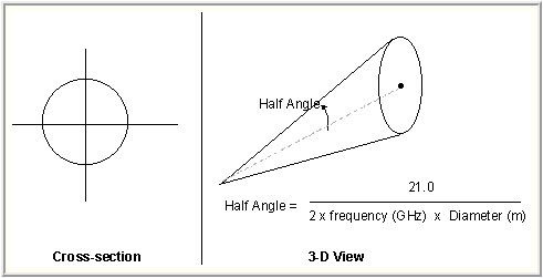
Half Power Sensor
- Open Servo_Motor's () Properties ().
- Select the Basic - Definition page in the Properties Browser.
- Open the Sensor Type drop-down list.
- Select Half Power.
- Enter the following specifications in the Half Power panel:
- Click to accept the changes and keep the Properties Browser open.
| Option | Value |
|---|---|
| Frequency | 1.7045 GHz |
| Diameter | 1.6 m |
Modeling a Targeted Sensor
The Targeted pointing type causes the sensor to point to other objects in the scenario.
- Select the Basic - Pointing page.
- Open the Pointing Type drop-down list.
- Select Targeted.
- Notice that Track Mode is set to Receive in the Targeted panel.
- Select TerraSarX_31698 () in the Available Targets list.
- Click move (
 ) to move TerraSarX_31698 () to the Assigned Targets list.
 - Click to accept the changes and to close the Properties Browser.
Calculating access
Use the Access tool to determine how often Servo_Motor can track TerraSarX_31698.
- Right-click on Servo_Motor () in the Object Browser.
- Select Access... (
 ) in the shortcut menu.
 - Select TerraSarX_31698 () in the Associated Objects list in the Access tool.
- Click
 .
. - Note the access intervals are now displayed in the Timeline View.
- Click to close the Access tool.
Viewing your progress
Use the Timeline View to see the access you created in the 3D Graphics window.
- Bring the 3D Graphics window to the front.
- Go to the Timeline View.
- Slowly move the Gray Pointer (
 ) until the sensor accesses the satellite.
 - Use your mouse to change the view so that you can view the access between Servo_Motor () and TerraSarX_31698 ().
![]()
Sensor Targeting Satellite
Modeling a Complex Receiver
Model a Complex Receiver on the sensor. The Complex Receiver model allows you to select among a variety of analytical and realistic antenna models, and to define the characteristics of the selected antenna type.
Inserting a Receiver
Attach a Receiver object to the Servo_Motor Sensor object.
- Insert a Receiver (
 ) object using the Insert Default () method.
 - Select Servo_Motor () in the Select Object dialog box.
- Click .
- Rename Receiver1 () to Download_Rx.
Setting the receiver model specs
Use a Complex Receiver Model.
- Open Download _Rx's () Properties ().
- Select the Basic - Definition page in the Properties Browser.
- Click the Receiver Model Component Selector ().
- Select Complex Receiver Model (
 ) in the Select Component dialog box.
 - Click to close the Select Component dialog box.
- Note that by default, the Frequency Auto Track is selected.
Frequency Auto Track allows a receiver to track and lock onto the transmitter's carrier frequency, with which it is currently linking, including any Doppler shift. LNA refers to Low Noise Amplifier. If you have those specifications, you can add them.
Defining the receiver antenna model
You can select to embed an antenna model from the Component Browser or you can link to an antenna object.
Use a parabolic antenna for your analytical model.
- Select the Antenna tab.
- Select the Model Specs sub-tab.
- Click the Antenna Model Component Selector ().
- Select Parabolic () in the Antenna Models list.
- Click to close the Select Component dialog box.
- Enter the following specifications:
- Click to accept the changes and keep the Properties Browser open.
| Option | Value |
|---|---|
| Design Frequency | 1.7 GHz |
| Diameter | 1.6 m |
Setting the receiver antenna polarization
The receiver polarization type is the same as the transmitter's polarization.
- Select the Polarization sub-tab.
- Select the Use check box.
- Open the Polarization drop-down list.
- Select Right-hand Circular.
- Click to accept the changes and close the Properties Browser.
Calculating a simple link budget
Creating a Link Budget in the Access tool is referred to as a Simple Link Budget. The Link Budget report is a specialized Access report for basic link budget analysis and is available using the Link Budget button in the Reports panel of the Access window.
- Right-click on Download_Rx () in the Object Browser.
- Select Access... () in the shortcut menu.
- Expand (
 ) TerraSarX_31698 () in the Associated Objects list in the Access tool.
 - Select Download_Tx ().
- Click in the Reports panel.
- Take some time to look at the Simple Link Budget report.
- Leave the Link Budget report open.
- Leave the Access tool open.
You should see six separate groups of access times. As the satellite rises over the horizon of the WGS84 central body ellisoid, you receive transmissions. When the satellite falls below the horizon, you lose transmissions.
Taking terrain into consideration
Use the Terrain Mask option to take the terrain into consideration for access. If this option is selected, access to the object is constrained by any terrain data in the line of sight to which access is being calculated.
- Open Download_Rx's () Properties ().
- Select the Constraints - Active page.
- Click Add new constraints (
 ) in the Active Constraints toolbar.
 - Select Terrain Mask in the Constraint Name list in the Select Constraints to Add dialog box.
- Click .
- Click to close the Select Constraints to Add dialog box.
- Click to accept the changes and close the Properties Browser.
Determining the effect of the terrain
Refresh the Link Budget report to see the effect of the terrain.
- Return to the Link Budget report.
- Click Refresh (F5) (
 ) in the report's toolbar.
 - Notice that all accesses blocked by analytical terrain (RaistingStation.pdtt) have been removed from the report.
- Close (
 ) the Link Budget report.
You began with six (6) groups of accesses but taking terrain into account you now have four (4) groups.
Generating a Detailed Link Budget report
The
- Return to the Access tool.
- Click .
- Select the Link Budget - Detailed (
 ) report in the Installed Styles (
 ) folder.
 - Click .
- Click at the top of the report.
- Enter 30 sec in the Step field.
- Select the Enter key.
- Take some time to look at the report.
- Note the values in the C/N (dB) (carrier to noise ratio), Eb/No (dB) (energy per bit to noise ratio), and BER (Bit Error Rate) columns.
- Leave the Detailed Link Budget report open.
Looking at the first access, note the values for Atmos Loss (dB) and Rain Loss (dB). They're currently zero (0). You haven't loaded any RF Environment models.
For the purposes of your analysis, due to downloading data, you require a BER equal to or lower than 1.000000e-13. You can see from the report that you only have a few minutes during each pass to download data.
Modeling rain
Environmental factors can affect the performance of a communications link. Apply rain and atmospheric absorption models to the analysis. Rain models are used to estimate the amount of degradation (or fading) of the signal when passing through rain.
- Open STK_Communications' () Properties ().
- Select the RF - Environment page.
- Select the Rain, Cloud & Fog tab.
- Select the Use check box in the Rain Model panel.
- Leave the default ITU (International Telecommunication Union) model.
- Click to accept the changes and keep the Properties Browser open.
Modeling atmospheric absorption
Atmospheric Absorption models estimate the attenuation of atmospheric gases on terrestrial and slant path communication signals.
- Select the Atmospheric Absorption tab.
- Select the Use check box.
- Leave the default ITU model.
- Click to accept the changes and close the Properties Browser.
Applying changes to the Detailed Link Budget report
Refresh the Detailed Link Budget report to see the environmental effects.
- Return to the Link Budget - Detailed report.
- Scroll to the C/N (dB), Eb/No (dB) and BER columns.
- Click Refresh (F5) () in the report's toolbar.
- Scroll to the Atmos Loss (dB) and Rain Loss (dB) columns.
- Leave the report open.
There was a slight change in the C/N (dB) and Eb/No (dB) values.
Losses were minimal in the C/N (dB) and Eb/No (dB) values.
Modeling System Noise Temperature
The Receiver's System Noise Temperature allows you to specify the system's inherent noise characteristics.
- Open Download_Rx's () Properties ().
- Select the Basic - Definition page in the Properties Browser.
- Select the System Noise Temperature tab.
- Select the Compute option.
- Select the Compute option in the Antenna Noise panel.
- Select the following options:
- Sun
- Atmosphere
- Rain
- Cosmic Background
- Click to accept the changes and close the Properties Browser.
Applying changes to the Detailed Link Budget report
Refresh the Detailed Link Budget report to see the effects of the noise characteristics.
- Return to the Link Budget - Detailed report.
- Scroll to the C/N (dB), Eb/No (dB) and BER columns.
- Click Refresh (F5) () in the report's toolbar.
- Look at the following columns in the report and observe their values:
- Tatmos (K)
- Train (K)
- Tsun (K)
- Tearth (K)
- Tcosmic (K)
- Tantenna (K)
- Tequivalent (K)
There were increases in the C/N (dB) and Eb/No (dB) values and decreases in BER.
These are the calculated noise temperatures. Calculating system noise temperature improved your Link Budget report and extended the time available for downloading data.
Saving your work
Clean up your workspace and save your scenario.
- Close any open reports, properties and tools.
- Save () your work.
Summary
You inserted a Place object into the scenario, which simulated the location of a scientific team monitoring glacial melt-water in mountainous terrain. You used a local terrain file both analytically and visually for your analysis and situational awareness. You inserted and propagated an Earth-observing Satellite object, which the scientists needed to communicate with for data download. You were introduced to the Simple Transmitter Model, which was attached to the Satellite object. The Simple Transmitter used an isotropic antenna. Next, you created a servo motor using a Sensor object, which was used to steer the ground site receiver antenna by locking onto the Satellite object. The Receiver object used a Complex Receiver Model. This model allowed you to input a parabolic antenna pattern. The first analysis, using the Access tool, focused on a Simple Link Budget. The only constraint applied was line of sight, which is basically horizon to horizon using the central body. Next, using Terrain Mask, you took into account local terrain and lost multiple accesses to the Satellite object. You moved to the Report & Graph Manager and generated a Detailed Link Budget. You enabled an ITU rain model and atmospheric absorption model, which had a slight detrimental impact on the Link Budget report. Finally, you added System Noise Temperature analysis to the Link Budget report, which had a positive impact to the link budget.
On your own
Throughout the tutorial, hyperlinks are provided, which point to in-depth information concerning Transmitter and Receiver objects. Now's a good time to go back through this tutorial and review that information.
For further study
With the STK software's Communications capability, you can model all the physical components of a system. Two important aspects are modulators and additional gains and losses.
Selecting another modulator
The STK application's Communications capability allows you to select from multiple modulators, including user-defined modulators. Each modulator has a defined modulation. Normally, you perform this function in the Transmitter object.
- Open the Transmitter object's () Properties ().
- Select the Modulator tab.
- To understand the settings on this page, click HERE.
Selecting a different demodulator
The Receiver object defaults to the same modulation as the Transmitter object when calculating a Link Budget report. However, you can override this behavior.
- Open the Receiver object's () Properties ().
- Select the Demodulator tab.
- To understand the settings on this page, click HERE.
Modeling additional gains and losses
During communications analyses, it is often necessary to model gains and losses that affect performance, but which are not defined using built-in analytical models. The STK software allows you to model these by specifying additional gains and losses that can be added to the equation. These can be added in both the Transmitter and Receiver objects.
- Select the Additional Gains and Losses tab.
- To understand the settings on this page, click HERE.