STK Premium (Air), STK Premium (Space), or STK Enterprise
You can obtain the necessary licenses for this tutorial by contacting AGI Support at support@agi.com or 1-800-924-7244.
Required Capability Install: For versions 12.10 and earlier of the STK software, this lesson requires the installation of the EOIR capability. For these versions of the software, the EOIR installer is included in the STK Premium software download, but requires a separate installation process. Read the Readme.htm found in the STK software install folder for installation instructions. You can obtain the necessary install by visiting https://support.agi.com/downloads or calling AGI support.
The results of the tutorial may vary depending on the user settings and data enabled (online operations, terrain server, dynamic Earth data, etc.). It is acceptable to have different results.
Capabilities covered
This lesson covers the following capabilities of the Ansys Systems Tool Kit® (STK®) digital mission engineering software:
- STK Pro
- Electro-Optical Infrared Sensor Performance (EOIR)
Problem statement
Engineers, mission planners, and operators need to determine when an airborne sensor system can detect, track, identify, and characterize targets of interest under operational conditions. You are conducting a test flight of a commercial space launch vehicle from a launchpad at Kennedy Space Center in Florida. You want to track the launch vehicle using an aircraft-mounted mid-wave infrared (MWIR) thermal imaging camera system as it travels along its arc. You want to be able to view the launch vehicle as it would appear in the MWIR camera, including both its body shape and the behavior of its exhaust plume, and to analyze the sensor data.
Solution
Use the STK software's Electro-Optical Infrared Sensor Performance (EOIR) to model an airborne mid-wave infrared observation system and a Missile object to define and build the launch vehicle's EOIR shape and simulate its exhaust plume. Then, generate a sensor scene that shows the launch vehicle and its exhaust plume as it traverses its arc. Optionally, export your EOIR sensor scene frames and stitch them together to create a video of the launch.
What you will learn
Upon completion of this tutorial, you will understand how to do the following:
- Use the EOIR capability to design an air-based EOIR observation system
- Model a mid-wavelength infrared camera
- Model a launch vehicle's EOIR shape using a Missile object
- Define the behavior and properties of a vehicle's exhaust plume
- Export EOIR sensor scene frames
- Create a video from individual still images of an EOIR sensor scene
Creating a new scenario
First, you must create a new STK scenario, and then build from there.
- Launch the STK application (
 ).
). - Click
 Create a Scenario in the Welcome to STK dialog box.
 - Enter the following in the STK: New Scenario Wizard:
- Click when you finish.
- Click Save (
 ) when the scenario loads.
 - Verify the scenario name and location in the Save As window.
- Click .
| Option | Value |
|---|---|
| Name | EOIR_AirObservation |
| Start | Default Date / Set Time to 16:00:00.000 |
| Stop | + 10 mins |
The STK application creates a folder with the same name as your scenario for you.
Save () often during this lesson!
Disabling streaming terrain
By default, the STK application connects to the Ansys Geospatial Data Cloud to distribute Earth terrain data for analysis and visualization. Turn off
- Right-click on EOIR_AirObservation () in the Object Browser.
- Select Properties (
 ) in the shortcut menu.
 - Select the Basic - Terrain page when the Properties Browser opens.
- Clear the Use terrain server for analysis check box in the Terrain Server panel.
- Click to confirm your change and to close the Properties Browser.
Modeling the test aircraft
Your airborne test platform consists of an EOIR sensor mounted to a high-altitude research aircraft. Start by modeling the aircraft and its route.
Inserting an Aircraft object
Insert an
- Bring the Insert STK Objects tool (
 ) to the front.
 - Select Aircraft (
 ) in the Select An Object To Be Inserted listed.
 - Select Insert Default () in the Select A Method list.
- Click .
- Right-click on Aircraft1 () in the Object Browser.
- Select Rename in the shortcut menu.
- Rename Aircraft1 () TestAcft.
Modeling the aircraft's route
For this scenario, you will model a quick, two-waypoint, high-altitude flight path for the aircraft to observe the space launch vehicle. Use the default
- Open TestAcft's () Properties ().
- Select the Basic - Route page when the Properties Browser opens.
- Note GreatArc is selected for the Propagator by default.
Inserting the route's waypoints
The waypoints that comprise the great arc route are contained in a table that displays each point, along with all of its properties, in sequence. You can use the table to directly edit those properties. One row of values describes a single waypoint in the route of the vehicle. Enter the two waypoints manually.
- Leave Smooth Rate set for the Route Calculation Method.
- Click .
- Enter the following values for the first waypoint by clicking in the associated cell:
- Select the Enter key.
- Click again.
- Enter the following values for the second waypoint:
- Select the Enter key.
- Click to confirm your changes and to close the Properties Browser.
This will use the Speed property of each waypoint to calculate the route between the waypoints.
| Latitude | Longitude | Altitude |
|---|---|---|
| 26.72 deg | -76.90 deg | 20.00 km |
| Latitude | Longitude | Altitude |
|---|---|---|
| 25.25 deg | -76.60 deg | 20.00 km |
Modeling the launch vehicle
Next, model the launch vehicle and its trajectory using a Missile object. While it may seem more intuitive to use a
Inserting a Launch Vehicle object
Insert a new Launch Vehicle object using the Define Properties method.
- Bring the Insert STK Objects tool () to the front.
- Insert a Launch Vehicle (
 ) object using the Define Properties () method.
 - Enter 25 m in the Launch Altitude field when the Properties Browser opens.
- Click to confirm your change, close the Properties Browser, and propagate the Launch Vehicle object.
You will be modeling a vehicle with a 50-meter tall body, and the launch altitude is measured from the model's center point. In order for the launch vehicle's EOIR shape to be positioned correctly, you must adjust this launch altitude accordingly.
Exporting the Launch Vehicle object's ephemeris
The Launch Vehicle object uses the
- Right-click on LaunchVehicle1 () in the Object Browser.
- Select Export Ephemeris/Attutide... in the shortcut menu.
- Click next to the Output File field when the Create Data File dialog box opens.
- Navigate your scenario folder (for example, C:\Users\<username>\Documents\STK_ODTK 13\EOIR_AirObservation) when the External Type dialog box opens.
- Note the File name is set to LaunchVehicle1.e.
- Click to confirm your selection and to close the External Type dialog box.
- Click to close the Create Data File dialog box.
- Clear the check box for LaunchVehicle1 () in the Object Browser.
You do not need to display it for further analysis.
Inserting a Missile object
Model the launch vehicle with a Missile object. A
- Bring the Insert STK Objects tool () to the front.
- Insert a Missile (
 ) object using the Insert Default () method.
 - Rename Missile1 () TestVehicle.
Importing the Launch Vehicle object's ephemeris
The
- Open TestVehicle's () Properties ().
- Select the Basic - Trajectory page when the Properties Browser opens.
- Open the Propagator drop-down list.
- Select StkExternal.
- Click the Filename ellipsis (
 ).
). - Navigate to your scenario folder (for example, C:\Users\<username>\Documents\STK_ODTK 13\EOIR_AirObservation) when the Select an Ephemeris File dialog box opens.
- Select LaunchVehicle1.e.
- Click to confirm your selection and to close the Select an Ephemeris File dialog box.
- Click to confirm your changes and to keep the Properties Browser open.
Building TestVehicle's EOIR shape
Set up the EOIR Shape for the launch vehicle. You can select shapes and specify corresponding dimensions to represent them. This will define what the sensor will see when it targets TestVehicle.
Adding the first component
A Missile object's
- Select the Basic – EOIR Shape page.
- Ensure Component1 is selected in the Component list.
- Open the Shape drop-down list.
- Select Cylinder.
- Enter the following dimensions for Component1:
- Leave the Body Temperature set to Static.
- Enter 500 K in the Temperature panel.
- Leave the Material set to Gray Body.
- Click to confirm your changes and to keep the Properties Browser open.
| Option | Value |
|---|---|
|
Height |
50 m |
| Radius | 10 m |
This temperature is applied the entire shape over the entire EOIR scene time period.
This is the
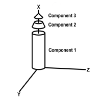
Component stacking orientation
Adding a second component
Now, create a second, conical component to model the launch vehicle's nose cone.
- Click next to the Component list.
- Set the following options for Component2:
- Click to confirm your changes and to keep the Properties Browser open.
| Option | Value |
|---|---|
|
Shape |
Cone |
|
Height |
50 m |
| Radius | 10 m |
| Body Temperature | Static |
| Temperature | 500 K |
When an object of one material consists of two or more simple geometric shapes, the EOIR capability will approximate each shape as a bounded sphere while estimating the percentage overlap for high-accuracy areas.
Defining TestVehicle's exhaust plume
TestVehicle launches with a three-minute burn. Use the
- Select the Basic – EOIR Stage page.
- Note the On Time Delta is set to 0 sec.
- Enter 180 sec in the Off Time Delta field.
- Click to confirm your changes and to close the Properties Browser.
This is the point in time at which the plume is turned on, specified in seconds from the start time.
This is the point in time at which the plume is shut off, specified in seconds from the start time. The minimum time is 0 sec and the maximum is 86,400 sec (one day).
Your launch vehicle has only a single stage. For multi-stage vehicles, you must create one Missile object for each stage.
Modeling the MWIR camera with EOIR
The
To create an EOIR scene, you need to specify the
Inserting a Sensor object
Attach a Sensor object to TestAcft. A
- Bring the Insert STK Objects tool () to the front.
- Insert a Sensor (
 ) object using the Insert Default () method.
 - Select TestAcft () when the Select Object dialog box opens.
- Click to insert the Sensor object and to close the Select Object dialog box.
- Rename Sensor1 () MWIR.
Updating the sensor's location
Place the sensor on the nose of the aircraft by updating its
- Open the MWIR's () Properties ().
- Select the Basic – Location page when the Properties Browser opens.
- Open the Location Type drop-down list.
- Select Fixed.
- Ensure Cartesian is selected in for the Type in the Fixed Location panel.
- Set the following Cartesian coordinates:
- Click to confirm your changes and to keep the Properties Browser open.
With a Fixed Location type, the location of the sensor is defined using a fixed displacement vector with respect to the parent object’s body frame.
| Option | Value |
|---|---|
| X | 0.018 km |
| Y | 0 km |
| Z | 0 km |
Targeting the sensor to TestVehicle
The camera tracks and follows TestVehicle. Update the sensor's
- Select the Basic – Pointing page
- Open the Pointing Type drop-down list.
- Select Targeted.
- Select TestVehicle () in the Available Targets list.
- Move (
 ) TestVehicle () to the Assigned Targets list.
 - Click to confirm your changes and to keep the Properties Browser open.
The Targeted pointing type causes the sensor to point to other objects in the scenario.
Selecting the EOIR sensor type
Select the EOIR sensor type on the sensor's
- Select the Basic - Definition page.
- Open the Sensor Type drop-down list.
- Select EOIR.
- Double-click in the Band name field.
- Rename the band MWIR.
- Click to confirm your changes and to keep the Properties Browser open.
Setting the sensor's spatial properties
By default, an EOIR sensor is set up with a single band. Select the Spatial tab on the Definition page to specify the spatial properties for each band. The default input setting for the band is Field-of-View and Number of Pixels. Update the sensor's field of view to narrow its focus.
- Select the Spatial tab.
- Leave Field-of-View and Number of Pixels selected for the Input method.
- Enter the following values in the Field of View panel
- Click to confirm your changes and to keep the Properties Browser open.
| Option | Value |
|---|---|
| Vertical Half Angle | 0.02 deg |
| Horizontal Half Angle | 0.02 deg |
The EOIR capability uses these half angles to determine the full angular extent of the sensor field of view (FOV).
Setting the sensor's spectral properties
Specify the sensor's
- Select the Spectral tab.
- Enter the following values in the Spectral Band Edge Wavelengths panel:
- Leave the Number of Intervals as the default.
- Leave the Spectral Shape set to the Use Optical and Radiometric Response option.
- Click to confirm your changes and to keep the Properties Browser open.
You must set the High value first.
| Option | Value |
|---|---|
| High | 5.50 |
| Low | 3.00 |
The internal sensor model samples your spectral band using the number of intervals you define. The more intervals you have, the higher the accuracy of the analysis. However, more intervals mean longer computation time.
This leaves the spectral shape to the individual optical transmission and quantum efficiency spectral characteristics.
Setting the sensor's optical properties
Next, specify the sensor's optical properties by choosing which two optical parameters will serve as the inputs used to calculate a third parameter.
- Select the Optical tab.
- Open the Input drop-down list.
- Select Focal Length and Entrance Pupil Diameter.
- Enter the following input parameters, which are measured in centimeters:
- Select Negligible Aberrations.
- Click to confirm your changes and to keep the Properties Browser open.
| Option | Value |
|---|---|
| Effective Focal Length | 415 |
| Entrance Pupil Diameter | 100 |
The EOIR capability models aberrations based on a root-mean-square wavefront error. The Negligible Aberrations setting introduces a 7% wave front error.
Setting the sensor's radiometric properties
The sensor's radiometric properties define its noise floor and its saturation ceiling.
- Select the Radiometric tab.
- Leave the Input set to High Level.
- Leave the Sensitivity values set at their default values.
- Click to confirm your changes and to close the Properties Browser.
With high-level radiometric parameters, you can populate and edit sensor performance data with measurements from an actual sensor or estimates for a sensor being developed.
When preparing to take measurements with a sensor model, you specify an integration time. This is the time interval over which a radiant signal is collected before generating an image. The longer the time, the more photons that get collected. This field is equivalent to the "exposure time" setting on an analog film camera. You can also define a set of points that relate Integration (Exposure) Time to NEI/SEI (noise equivalent irradiance / saturation equivalent irradiance). The STK application linearly interpolates between the points to get correct NEI/SEI for the integration time you set.
Viewing the setup in the 3D Graphics window
Take a look at your setup in the 3D Graphics window to gain situational awareness.
- Right-click on TestVehicle () in the Object Browser.
- Select Zoom To in the shortcut menu.
- Bring the 3D Graphics window to the front.
- Use your mouse to zoom out and get a good view of the relationship between the launch site, TestVehicle, TestAcft, and the sensor field of view.
Setting the animation time
TestVehicle will launch from the ground with a three-minute burn duration. To make it easier to see, move forward in the scenario by a few seconds.
- Click Decrease Time Step (
 ) on the Animation toolbar until the Time Step is set to 1.00 sec.
 - Click Start (
 ) on the Animation toolbar.
 - Watch as TestVehicle lifts off from the launch pad and is tracked by the MWIR sensor.
- Click Reset (
 ) on the Animation toolbar when finished.
 - Click Step Forward (
 ) on the Animation toolbar to move ahead to three seconds after TestVehicle's burn starts.
Opening the EOIR toolbar
To
- Select View in the Menu Bar.
- Select Toolbars in the View menu.
- Select EOIR in the Toolbar submenu to show the EOIR toolbar (
 ).
).
Updating the EOIR configuration
To see TestVehicle in the EOIR sensor scene, you must first add it as a target in the EOIR configuration. When you include an object as a target in the EOIR configuration, its EOIR properties are taken into account.
- Click EOIR Configuration... (
 ) on the EOIR toolbar.
 - Select Missile/TestVehicle () in the Available STK Objects list when the EOIR Configuration dialog box opens.
- Move (
 ) Missile/TestVehicle () to the Selected Targets list.
 - Click to confirm your selection and to close the EOIR Configuration dialog box.
All central bodies and objects, except for the source sensor, that are part of the EOIR Configuration are listed in the Available STK Objects list.
An EOIR sensor will take images of objects in the Selected Targets list that are sufficiently bright, either in reflected light or from self-radiance, at wavelengths that the sensor can detect.
Generating an EOIR sensor scene
Now you are ready to
Generating the sensor scene from the EOIR toolbar
To generate an input scene for the selected sensor, use the buttons on the EOIR toolbar.
- Select MWIR () in the Object Browser.
- Click EOIR Sensor Scene... (
 ) on the EOIR toolbar.
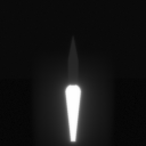
TestVehicle and exhaust plume
The
Adjusting and reviewing the simulated scene
Open the
- Right-click on the sensor scene.
- Select Details... in the shortcut menu.
- Move the EOIR Scene Visual Details dialog box when it opens so that it's not sitting on top of the sensor scene.
- Click on TestVehicle's body and on its exhaust plume in the EOIR sensor scene.
- Select the Fine option in the Scene Detail panel.
- Select the BGRY option in the Color Map panel.
- Click to confirm your changes and to close the EOIR Scene Visual Details dialog box.
- Keep the EOIR Sensor Scene window open.
Note that, in addition to the name of the Missile object (TestVehicle), other information about the vehicle is displayed in the Scene Pick Information panel in the EOIR Scene Visual Details dialog box, including the distance to it in kilometers, the azimuth and elevation to the target, and the thermal model temperature and material type of the surface location. You can see that both the body and exhaust plume are defined as Gray Body materials with the temperatures specified in TestVehicle's EOIR Shape and Stage properties, respectively.
Selecting a color map enables various "false color" mappings of the display. EOIR uses false color to bring out details in the image data that are often lost when displayed on a monitor with less resolution than the EOIR sensor. For instance, a typical monitor can display only 256 levels of grayscale, whereas an EOIR sensor might have 4096 levels of grayscale resolution. Color mapping is only for visual effect and does not change any of the internal data values. This can be particularly useful when viewing materials of differing temperatures through an infrared sensor.
Examining an event
TestVehicle executes a burn for the first three minutes of its flight. View what the sensor is seeing the moments before and after the burn ends.
- Manually change the Current Scenario time in the Animation toolbar so that it is two minutes and 59 seconds after your scenario start time (for example, 16:02:59.000).
- Select the Enter key.
- Bring the EOIR Sensor Scene window to the front.
- Examine your EOIR sensor scene.
- Click Step Forward () to move ahead to one second after the end of TestVehicle's burn.
- Examine your EOIR sensor scene and note the changes.
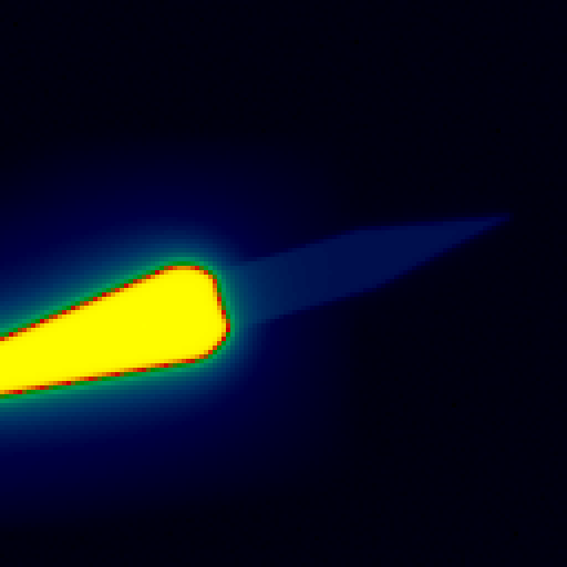
TestVehicle and exhaust plume BGRY COLOR MAP
You should see TestVehicle and its plume. Note the radiant glow from the heat produced by the plume.
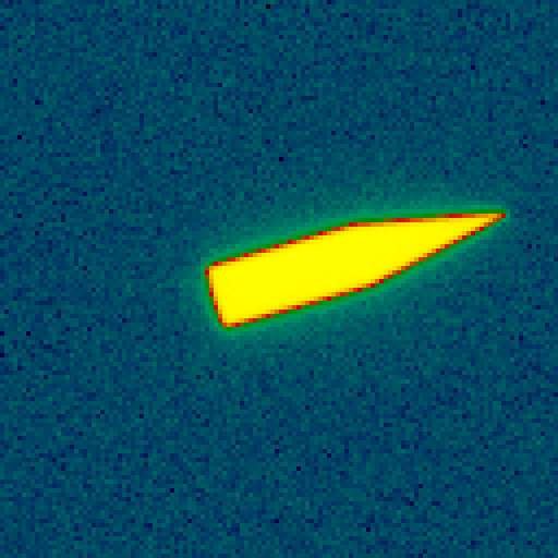
TestVehicle exhaust plume off
Note that the test vehicle continues to emit a radiant glow even after the burn stops, owing to the temperature of the body components. Also note that the background has changed. This is because your sensor scene has Automatic Gain Control (AGC) enabled. With this selection, the EOIR capability automatically calculates brightness and contrast such that the brightest scene detail fits within the brightness resolution of the monitor. At this moment in time, there is no burn, so the leveling for the noise in your synthetic scene is also updated.
Adjusting TestVehicle's EOIR properties
Now that you’ve taken a look at TestVehicle, see how the system is affected when the launch vehicle's EOIR properties change.
Updating a component's temperature
Increase the temperature of one of TestVehicle's components to see how that changes your EOIR sensor scene.
- Open TestVehicle's () Properties ().
- Select the Basic - EOIR Shape page when the Properties Browser opens.
- Enter 1000 K in Component1's Temperature field.
- Click to confirm your change and to keep the Properties Browser open.
- Bring the EOIR Sensor Scene window to the front.
- Review the changes.
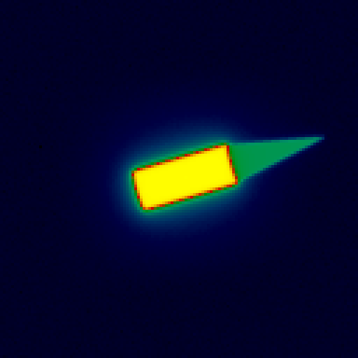
differing EOIR component temperatures
The sensor scene automatically regenerates based on the property updates when it is open. Note that TestVehicle's body is now glowing much brighter than its nose cone, as it is radiating more thermal energy.
Changing a component's surface material
The EOIR capability
- Return to TestVehicle's () Properties ().
- Enter 500 K in Component1's Temperature field.
- Open the Material drop-down list.
- Select Aluminum MLI.
- Click to confirm your changes and to keep the Properties Browser open.
- Bring the EOIR Sensor Scene window to the front.
- Review the changes.
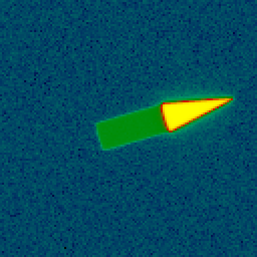
differing EOIR material types
In spite of the body temperature being the same between the two components, the body's aluminum multilayer insulation surface is radiating less heat.
Resetting the component's surface material
Reset the component's surface material back to Gray Body.
- Return to TestVehicle's () Properties ().
- Open the Material drop-down list.
- Select Gray Body.
- Click to confirm your changes and to close the Properties Browser.
- Keep the EOIR Sensor Scene window open.
Generating a custom EOIR graph
The EOIR capability does more than simulate scenes created by an EOIR sensor. Its internal sensor model can also calculate metrics a sensor would receive from a target's signal. Use the
Creating a custom graph style
First, create a new graph style called EOIR_TargetRadiance.
- Right-click on MWIR () in the Object Browser.
- Select Report & Graph Manager... in the shortcut menu (
 ).
). - Select the My Styles (
 ) folder in the Styles panel when the Report & Graph Manager opens.
 - Click Create new graph style (
 ) on the Styles toolbar.
 - Name the graph style EOIR_TargetRadiance.
- Select the Enter key to rename the graph style and open the Properties Browser.
Selecting the graph's data providers
Use the
- Expand (
 ) the EOIR Sensor To Target Metrics () data provider in the Data Provider list when the Properties Browser opens.
 - Select In-band target radiance (
 ) in the Data Provider list.
 - Move () the In-band target radiance () data provider element to the Y Axis list.
- Click to confirm your change and to close the Properties Browser.
These are time dependent metrics for a unique EOIR Sensor-Band / Target pairing.
Setting the graph's Time properties
Set the graph's
- Select the Specify Time Properties option in the Time Properties panel.
- Open (
 ) the Start and Stop times drop-down menu.
 - Select Interval Component....
- Select TestVehicle () in the Objects list when the Select Time Interval dialog box opens.
- Select EphemerisTimeSpan (
 ), located in the Installed Components () folder, in the Intervals for: TestVehicle list.
 - Click to confirm your selection and to close the Select Time Interval dialog box.
Generating the Sensor to Target Metrics graph
Now, generate the EOIR Target Radiance graph over the duration of the burn.
- Select the Use step size/ time bound option.
- Enter 10 sec in the Step size field.
- Select Sensor to Target Metrics (
 ) in the Styles list.
 - Click .
- Review the graph.
- Hover your mouse over the radiance values after the burn has ended to examine their levels.
- Close your Sensor to Target Metrics graph when finished.
- Click to close the Report & Graph Manager.
- Save () your scenario.
Be patient. It may take the STK application a while to generate the graph.
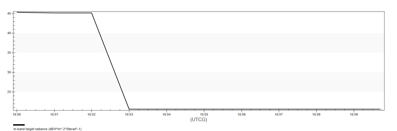
TestVehicle exhaust plume off
Note the drop in target radiance when TestVehicle's burn ends around the three-minute mark.
Creating a video from saved EOIR images
You can create a video from your EOIR images using free or professional video editing software. Configure your scenario to export EOIR frames at an appropriate format and frame rate.
This is an optional section for those who wish to learn how to create a video for EOIR sensor scenes if you do not want to create a video, skip to the Saving your work section.
Updating the scenario’s Basic Time properties
For the purposes of this tutorial, you want to make a ten-second movie, beginning five seconds before and after the burn ends. Update the scenario's
- Open EOIR_AirObservation's () Properties ().
- Select the Basic - Time page when the Properties Browser opens.
- Clear the Use Analysis Start Time check box in the Animation panel.
- Set the Start time to five seconds before the burn ends, for example, [date] 16:02:55.000.
- Select the Stop at Time check box.
- Clear the Use Analysis Stop Time check box.
- Set the Start time to fives seconds after the burn ends, for example, [date] 16:03:05.000.
- Enter 0.03 seconds in the Step Size field.
- Click to confirm your changes and to close the Properties Browser.
- Click Reset () on the Animation toolbar.
This is equivalent to approximately 30 frames per second (fps), a standard digital video content frame rate.
Preparing your sensor scene
The EOIR capability processes the raw sensor data or a scene bitmap (*.bmp) based on the selected level (radiometric input, geometric input, or sensor output) for each animation time step.
- Right-click on the sensor scene in the EOIR Sensor Scene window.
- Select Details... in the shortcut menu.
- Move the EOIR Scene Visual Details dialog box when it opens so that it's not sitting on top of the sensor scene, if needed.
- Select the Scene Bitmap check box in the Automatic File Output panel.
Setting the storage location
Images are saved as BMP files in the specified folder location.
- Click the Storage Location ellipsis ().
- Right-click in the folder and file browser when the storage location dialog box opens.
- Ensure you are in your scenario folder (for example, C:\Users\<username>\Documents\STK_ODTK 13\EOIR_AirObservation).
- Select New in the shortcut menu.
- Select Folder in the New submenu.
- Name your folder EOIR_Movie.
- Select the Enter key.
- Ensure EOIR_Movie is noted in the Folder field.
- Click to confirm your selection and to close the storage location dialog box.
- Click to confirm your changes and to keep the EOIR Scene Visual Details dialog box open.
Note the Storage Location now points to your EOIR_Movie subfolder.
Creating the still frames
With your animation time and your output configured, capture your still frames.
- Click Start () on the Animation toolbar.
- Watch as the sensor scene animates in the EOIR Sensor Scene window.
- Return to the EOIR Scene Visual Details dialog box when the scenario has finished animating.
- Clear the Scene Bitmap check box in the Animation panel.
- Click to confirm your changes and to close the EOIR Scene Visual Details dialog box.
You don't want to capture every frame if you want to continue exploring your scenario.
Reviewing the results
When creating automatic file output for each animation step, the EOIR capability creates a new file with a file name that contains the corresponding time in epoch seconds.
- Open Windows File Explorer.
- Navigate to the location of your saved stills (for example, C:\Users\<username>\Documents\STK_ODTK 13\EOIR_AirObservation\EOIR_Movie).
- Look at your stills.
You can see you have over 300 stills for your short movie. Each is named with the name of the sensor and the time step it represents. This makes it easy to put them in sequential order.
Creating a new video project with the OpenShot Video Editor
You can use any number of video editing software choices to create your video, such as Adobe Premier or Microsoft ClipChamp. The steps that follow use the OpenShot Video Editor, a free and open-source video editor for Linux, Mac, and Windows. While the precise steps may be different in other editors, the concept is the same.
- Open the OpenShot Video Editor application.
- Click New Project on the Toolbar.
- Click Import Files.
- Navigate to the location of your saved stills (for example, C:\Users\<username>\Documents\STK_ODTK 13\EOIR_AirObservation\EOIR_Movie) when the Import Files... dialog box opens.
- Multi-select all 300+ stills in the folder.
- Click to confirm your selection and to close the Import Files... dialog box.
Be patient. This could take a while.
Building your video
With your stills added to your project's files, add them to the project Timeline.
- Multi-select all the images in the Project Files tab.
- Right-click on one of the images.
- Select Add to Timeline in the shortcut menu.
- Enter 0.03 in the Image Length (seconds) field in the Timeline Location panel when the Add To Timeline dialog box opens.
- Note the Total Length of your movie is calculated as 00:00:10.02 seconds.
- Click to confirm your changes and to close the Add To Timeline dialog box.
- Click Play in the Video Preview panel to ensure your video looks correct.
Set this value based on the time step the images were taken in the scenario.
The Track has an initial time of 00:00:00,01.
Be patient. This may take a while. The images should automatically be added to the timeline based on their files names, which, as you recall, reflect the time steps you specified.
Exporting your video
With your frames put in order and displaying for an appropriate amount of time, export a video out of your project.
- Click Export Video on the toolbar.
- Enter EOIR_Movie in the File Name field when the Export Video dialog box opens.
- Click next to the Folder Path field.
- Set the Folder Path to where you saved your stills (for example, C:\Users\<username>\Documents\STK_ODTK 13\EOIR_AirObservation\EOIR_Movie) when the Choose a Folder... dialog box opens.
- Click to confirm your selection and to close the Choose a Folder... dialog box.
- Ensure the Target is MP4 (h.264).
- Ensure the Video Profile is HD 720p 30 fps (1280x720).
- Click .
- Click when the process is finished to close the Export Video dialog box.
Viewing your finished movie
Take a look at your finished movie.
- Return to Windows File Explorer.
- Open your finished MP4 movie with the video player of your choice.
- Watch as TestVehicle's burn stops in real time and the sensor gain levels change, just as you might see in a real EOIR sensor feed.
- Close the video player when you are finished.
If your movie does not look right — dropped frames, uneven animation, and so on, try exporting the video with different settings. For example, try exporting with a different video profile with a lower frame rate (such as 25 fps).
Resetting the scenario's Animation properties
Reset your scenario's animation time for the full analysis period.
- Close the OpenShot Video Editor when you are finished without saving your project.
- Return to the STK application.
- Open EOIR_AirObservation's () Properties ().
- Select the Basic - Time page when the Properties Browser opens.
- Select the Use Analysis Start Time check box in the Animation panel.
- Select the Use Analysis Stop Time check box.
- Click to confirm your changes and to close the Properties Browser.
Saving your work
Close out your scenario and save your work.
- Close (
 ) the EOIR Sensor Scene window.
 - Close any open reports, properties, and the Report & Graph Manager.
- Save () your work.
Summary
In this tutorial, you learned how to build and analyze an observation system on an aircraft. You tracked a launch vehicle using an EOIR sensor to see what a camera on the aircraft would see and even generated data from the sensor scene and from available EOIR data providers. This is especially useful information because you can see from your radiance graph that the signal is high during the initial burn, but drops once the burn completes. Your ability to track and detect objects like space launch vehicles depends on the sensors you design and build for your missions.
On your own
Expand your mission. In this lesson, you modeled a single sensor and a single band. The EOIR capability gives you the flexibility to model multiple sensors and bands for your mission. Try it out and see how your results may differ when looking at different parts of the spectrum.