Part 2:
STK Pro, STK Premium (Air), STK Premium (Space), or STK Enterprise
You can obtain the necessary licenses for this tutorial by contacting AGI Support at support@agi.com or 1-800-924-7244.
The results of the tutorial may vary depending on the user settings and data enabled (online operations, terrain server, dynamic Earth data, etc.). It is acceptable to have different results.
This tutorial requires version 12.9 of the STK software or newer.
Capabilities covered
This lesson covers the following capabilities of the Ansys Systems Tool Kit® (STK®) digital mission engineering software:
- STK Pro
Problem statement
Engineers and operators need to quickly add realistic analytical and visual properties to objects in the STK application. They may need a realistic satellite attitude, analysis of an enclosed area in a deep canyon, a mission plan for an aircraft flight route, a sensor footprint, or a briefing with detailed visuals and analysis.
Solution
Use the STK software to insert STK objects into your scenario. Then update the objects' properties to define their characteristics that are relevant to your scenario.
What you will learn
Upon completion of this tutorial, you will be able to:
- Update the STK software's databases
- Insert objects into your STK scenario
- Modify properties
- Understand why you are using different objects in your analysis
There are many objects and properties used in the STK software. Not all objects or properties are covered in this lesson. Other tutorials cover some objects or properties not discussed in this tutorial.
Video guidance
Watch the following video. Then follow the steps below, which incorporate the systems and missions you work on (sample inputs provided).
Data Update Utility
If you have an internet connection, you can use the Data Update Utility to update astro datasets such as EOP, Space Weather, Leap Second, time.ker, Solar Flux, satellite databases, GPS, etc. You can manually update one or more datasets, or you can schedule a time and frequency for automatic updates.
If you work with satellites, update your databases prior to opening a new scenario.
- Launch the STK application (
 ).
). - Extend the Utilities menu.
- Select the Data Update... option.
The color of the data set indicates its current status: red data sets have updates available, black are up to date, and purple are not currently available on AGI servers (these are rarely seen). If you select the Enable Automatic Updates check box, you can set your preferred options. Your PC needs to be on and connected to the Internet for the auto updates to occur.
- Select all the dataset check boxes that have updates available (Red) in the Update Column. Ignore black and purple datasets.
- Click .
- Click when the warning appears.
- Wait for the progress bar in the lower-right corner of the tool to complete and for all the datasets to turn black.
- Click when the update is complete to close the Data Update Utility.
- Click
 Exit STK in the Welcome to STK dialog box.
Creating a new scenario
Create a new scenario using the following steps. For a more detailed guide to creating a new scenario, see Lesson One: Build Scenarios.
- Launch the STK application ().
- Click
 Create a Scenario in the Welcome to STK dialog box.
 - Enter the following in the STK: New Scenario Wizard:
- Click when you finish.
- Click Save (
 ) when the scenario loads. The STK software creates a folder with the same name as your scenario for you.
 - Verify the scenario name and location in the Save As dialog box.
- Click .
| Option | Value |
|---|---|
| Name | STK_Objects_Properties |
| Location | Default |
| Start | Default |
| Stop | Default |
Modifying the Scenario object's properties
The Scenario (![]() ) object defines the context that influences the properties and behavior of other objects.
) object defines the context that influences the properties and behavior of other objects.
- Right-click on the Scenario () object in the Object Browser.
- Select Properties (
 ).
).
When the Scenario (![]() ) object's properties open, there is a branching list on the left containing pages of properties. The main category that you will need to know is the Basic category, which holds properties such as Time, Units, Database, and many others.
) object's properties open, there is a branching list on the left containing pages of properties. The main category that you will need to know is the Basic category, which holds properties such as Time, Units, Database, and many others.
Basic Time
In the Basic - Time page, the Analysis Period defines the epoch and the start/stop times for your scenario. Animation properties control the animation cycle, step duration, and the intervals between refresh updates in the graphics windows.
Throughout the various STK software tutorials, you are instructed to go to a properties page. Just click the specified page on the left.
Basic Units
Scenario Units establish the default settings for all units of measure used in a scenario.
- Select the Basic - Units page.
- Change the unit of any dimension listed in the table by clicking the CurrentUnit, such as kilometers (km), and selecting the appropriate value from the drop-down list.
Basic Database
Database properties enable you to set the defaults for the city, facility, satellite, and star databases. You can specify a stock STK database or one of your own that meets the STK software's format requirements.
Basic Earth Data
Use this page to update the Earth Orientation Parameters (EOP).
Basic Terrain
You can use the Terrain properties page of a scenario to enable streaming terrain. This enables you to view terrain features in the 3D Graphics window.
To use analytical terrain in your scenario requires an STK Pro license or higher.
- Select the Basic - Terrain page.
- Take a look around the Terrain page.
In the Terrain page, you should see the "Use terrain server for analysis" option. You can toggle the Terrain Server on and off with this option. "Advanced Analysis Operations" and "Custom Analysis Terrain Sources" require an STK Pro license.
Basic 3D Tiles
Version 12 of the STK software added the ability to include 3DTileset geometry (e.g., massive city models, photogrammetry, etc.) computationally in your analysis. The constraint 3DTiles Mask is available for Facility, Target, and Place objects as well as all vehicle types. You can apply 3D Tileset geometry to access calculations to determine obstructions due to terrain and stationary objects. You can use a 3D Titleset hosted on servers registered through Data Services, like Cesium ion, or stored on your local file system, for analysis.
Basic Global Attributes
Use the Basic - Global Attributes page to configure the display of warning messages for satellite and missile objects. By selecting the Basic - Global Attributes page, you should see options to suppress warnings for Satellites and Missiles.
Description
The Description page for an object is a handy place to record miscellaneous information about the object and its role in your analytical or operational task. By selecting this property, you should see a text box for a "Short Description," a larger text box for a "Long Description," and an area to add "Metadata."
Global Attributes
Global Attributes can (or, in some cases, must) be set at the scenario level for all objects.
2D Graphics Global Attributes
2D Graphics Global Attributes answer three basic questions about an STK object:
- What do you want to show?
- How do you want it to look?
- When do you want it to be seen?
Open the page to view the layout.
- Select the 2D Graphics - Global Attributes page.
- Take a look at the Global Attributes page, where you can decide what to display in the 2D and 3D Graphics windows.
There are a couple of things to keep in mind when using this page. Any changes you make on the Global Attributes page are applied to ALL objects that fall into the category (e.g., Vehicles). Any changes made on this page are also applied to 3D Graphics. For instance, if you disable the Show Labels option, object labels in both the 2D Graphics and 3D Graphics windows will be removed.
3D Graphics Global Attributes
You can use the 3D Graphics - Global Attributes properties page of a scenario to define 3D visualization options that affect the entire scenario.
- Select the 3D Graphics - Global Attributes page.
- Make note of the fields and what they do.
| Option | Description |
|---|---|
| Surface Reference of Earth Globes | Use either Mean Sea Level or WGS84 Ellipsoid (default). |
| 3D Object Editing | Enables you to pull great arc vehicles, facilities, and targets below the globe's surface reference — thus assigning them negative altitude values — while using 3D object editing. |
| Image Cache | Temporarily stores imagery for the globe. You may need to increase the size of the cache if all of the images that you are trying to display cannot be loaded at the same time or if an image appears blurry. |
| Terrain Cache | Temporarily stores terrain data for the globe. You may need to increase the size of the cache if all of the terrain that you are trying to display cannot be loaded at the same time or if the globe surface at the terrain level appears blurry. |
| Surface Lines | Enables you to select an option for displaying lines on the surface of the central body when terrain data is available. Select When Terrain Server is on to display surface lines on terrain only when you are connected to a terrain server, On to display surface lines on terrain data whenever it is available from any source, or Off to never display surface lines on terrain. |
2D and 3D Graphics Fonts
- Select the 2D Graphics - Fonts page.
- Select the 3D Graphics - Fonts page.
- Click to close the STK_Objects_Properties () Properties Browser.
2D Graphics Fonts enables you to configure the display of small, medium, and large fonts in your 2D Graphics window and apply an outline to the text to improve readability on changing map colors.
3D Graphics Fonts allows you to configure the display of small, medium, and large fonts in your 3D Graphics window and apply an outline to the text to improve readability on changing globe colors.
Insert STK Objects tool
The Insert STK Objects tool provides an easy, convenient way to populate a scenario. The Insert STK Objects tool, by default, displays the most commonly-used scenario objects. You can customize the tool to display all the scenario objects or a user-defined subset of objects.
- Click on the Insert STK Objects tool.
- Click Insert Object (
 ) located in the Default toolbar.
 - Expand the Insert menu and select New.
- Reopen the Insert STK Objects tool by using one of the aforementioned methods.
There are two ways to reopen the Insert STK Objects tool:
New object preferences
You can set preferences for the Insert STK Objects tool and setting default methods for inserting objects.
- Click in the Insert STK Objects tool.
- To choose the objects you want to appear in the Insert STK Objects tool, select the Show check box for them in the Object list.
- Click .
For the purposes of this tutorial, you won't make changes to the Object list. Later, you can enable all available objects and practice with them.
Objects and Methods
In the Insert STK Objects tool, you will see Scenario Objects, Attached Objects, and Methods. Scenario objects are children of the larger Scenario (![]() ). Attached objects are the children of scenario objects. You must add scenario objects before you can add attached objects.
). Attached objects are the children of scenario objects. You must add scenario objects before you can add attached objects.
To insert an object, you must choose a particular method. These methods determine the starting properties of each object. You can change these properties later. For instance, when this tutorial says to "Insert a Default Object," that means insert an object using the Insert Default method. You should pick the method for the demands of your scenario, as you will do later in this tutorial.
For instance, you could insert an Aircraft (![]() ) object (a Scenario object) using the Insert Default method. Then, you could insert a Sensor (
) object (a Scenario object) using the Insert Default method. Then, you could insert a Sensor (![]() ) object (an Attached object) onto that aircraft.
) object (an Attached object) onto that aircraft.
Scenario-level objects
The following Scenario Level objects will be discussed:
- Aircraft (
 )
)
- Area Target (
 )
)
- Facility (
 )
)
- Ground Vehicle (
 )
)
- Missile (
 )
)
- Place (
 )
)
- Satellite (
 )
)
- Ship (
 )
)
- Target (
 )
)
This tutorial doesn't cover every insert method for every object, but does cover different insert methods for different objects, to give you an idea what they do. Furthermore, the tutorial doesn't cover all properties. For instance, it describes some properties for the Aircraft (![]() ) object that you can apply to other objects.
) object that you can apply to other objects.
Satellite object
The Satellite object models the properties and behavior of a vehicle in orbit around a central body.
Inserting using From Standard Object Database method
- Select Satellite () in the Insert STK Objects tool.
- Select the From Standard Object Database (
 ) method.
 - Click .
- In the Name or ID field, enter 25544 (the SSC number or Satellite Catalog Number).
- Click .
- In the Results field, select ISS (Zarya).
- Click .
- Click to close the Search Standard Object Data window.
Both the satellite database file and the corresponding TLE file evolve over time and need to be updated.
The U.S. Strategic Command (USSTRATCOM) keeps track of thousands of space objects. These objects constitute the space object catalog. While most of the catalog is made available to the public, some information is restricted. AGI provides the publicly released information for use with the STK software in the form of satellite database files and two-line mean element files (TLEs).
The ISS (Zarya) is downloaded from AGI's Standard Object Data Service. If you were to choose ISS or Zarya from the Local Database, you would need to ensure you've updated your satellite database.
Viewing in 2D
- Bring the 2D Graphics window to the front.
- Zoom Out (
 ) if needed to see the entire earth and the current orbit track of ISS_ZARYA_25544 ().
 - Using the Animation Toolbar, make any adjustments to the time step.
- Click Start (
 ) to animate the scenario.
 - When finished, click Reset (
 ).
).
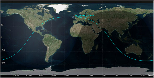
International Space Station Orbit in 2D
Viewing in 3D
- Bring the 3D Graphics window to the front.
- Click Home View (
 ).
). - Right-click on ISS_ZARYA_25544 () in the Object Browser.
- Select Zoom To.
- Using the Animation Toolbar, you can make adjustments to the time step.
- Click Start () to animate the scenario.
- When finished, click Reset ().
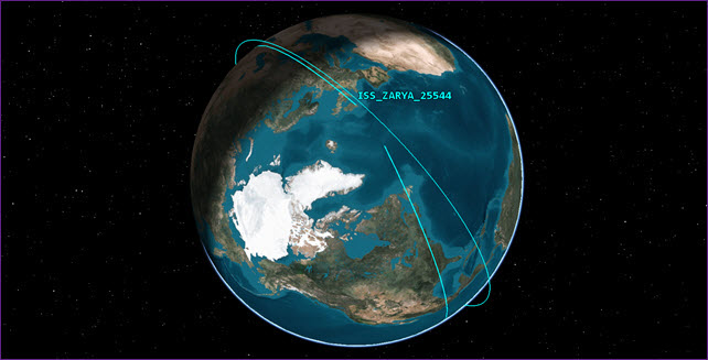
International Space Station Orbit in 3D
In this view, you can see both a ground track representing the ISS's current orbit and the actual orbit track. Not all Satellite (![]() ) objects are represented by both a ground track and an orbit track.
) objects are represented by both a ground track and an orbit track.
Using Real-time Animation Mode
The scenario animates in real time in accordance with your computer's internal clock. To visualize ISS_ZARYA_25544 (![]() ) using real-time animation mode, your scenario analysis period must fall within your current time. For instance, if the analysis period is set at 1 Jun 2020 18:00:00.000 UTCG - 2 Jun 2020 18:00:00.000 UTCG, and the actual local time is 1 Jun 2020 11:00 Mountain Time (11:00 am), ISS_ZARYA_25544 (
) using real-time animation mode, your scenario analysis period must fall within your current time. For instance, if the analysis period is set at 1 Jun 2020 18:00:00.000 UTCG - 2 Jun 2020 18:00:00.000 UTCG, and the actual local time is 1 Jun 2020 11:00 Mountain Time (11:00 am), ISS_ZARYA_25544 (![]() ) is not be visible. 1 Jun 2020 18:00:00.000 UTCG is 1 Jun 2020 12:00 local time. You'll have to adjust your scenario times if you experience this problem. If you do adjust your times, other moving objects such as the Aircraft (
) is not be visible. 1 Jun 2020 18:00:00.000 UTCG is 1 Jun 2020 12:00 local time. You'll have to adjust your scenario times if you experience this problem. If you do adjust your times, other moving objects such as the Aircraft (![]() ) object need to be readjusted too.
) object need to be readjusted too.
- Ensure that your scenario analysis period falls within your local time period.
- In the Animation Toolbar, select Real-time Animation Mode (
 ).
). - Click Start (). You're now visualizing ISS_ZARYA_25544 () at its actual location based on the TLE from which it was propagated.
- When finished, click Reset ().
- In the Animation Toolbar, select Normal Animation Mode (
 ).
). - Click Reset ().
Viewing ISS_ZARYA_25544's properties
- Right-click on ISS_ZARYA_25544's () in the Object Browser.
- Select properties ().
- The Propagator is set to the SGP4 Propagator. The STK software uses the Simplified General Perturbations (SGP4) Propagator with two-line mean element (TLE) sets.
- In the TLE Source panel, click Preview.... Here, you can preview or modify the two-line element (TLE) information that the STK software uses to propagate the SGP4 satellite.
- the TLE Preview window.
- Click to close ISS_ZARYA_25544's () Properties ().
Using Orbit Wizard
The Orbit Wizard is a satellite-level tool designed to assist you in either creating any one of several standard orbits or designing your own satellite orbit. The configurable options available depends on the orbit type selected.
- Select Satellite () in the Insert STK Objects tool.
- Select the Orbit Wizard (
 ) method.
 - Click .
- When the Orbit Wizard opens, set the following:
- Click .
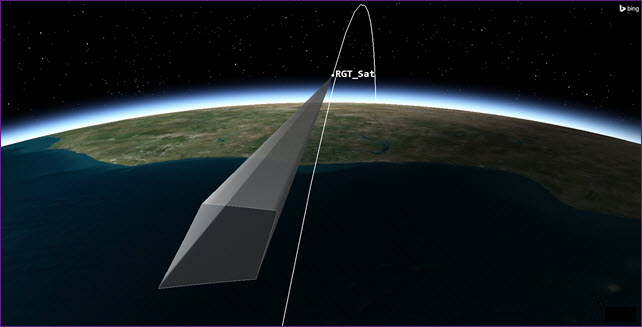
- Just like you did with ISS_ZARYA_25544 (), view RGT_Sat () in the 2D Graphics and 3D Graphics windows.
- Click Start () to animate the scenario.
- When finished, click Reset ().
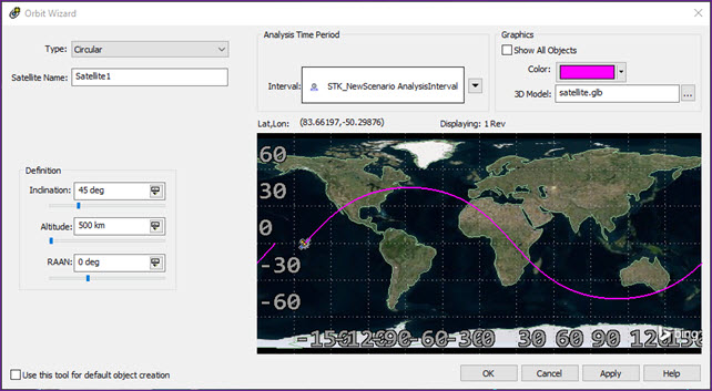
Orbit Wizard
| Option | Value |
|---|---|
| Type | Repeating Ground Trace |
| Satellite Name | RGT_Sat |
| Approximate Altitude | 600 km |
The Analysis Time Period / Interval defaults to your scenario analysis period. The satellite is propagated for that period.
Viewing RGT_Sat's properties
- Right-click on RGT_Sat () in the Object Browser.
- Select properties ().
- You can see that the propagator is set to J2 Perturbation.
Unlike a Satellite (![]() ) object propagated using TLEs, you can edit a Satellite (
) object propagated using TLEs, you can edit a Satellite (![]() ) object propagated using the Orbit Wizard using your own data.
) object propagated using the Orbit Wizard using your own data.
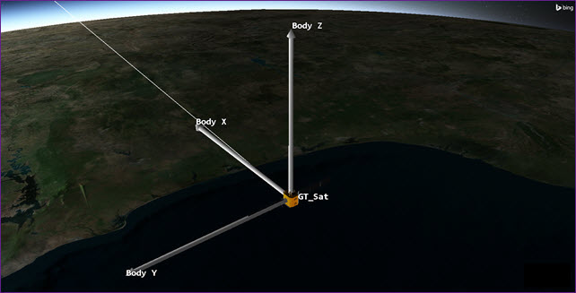
Showing satellite vectors and attitude
Sometimes you need to understand your attitude.
- Return to RGT_Sat's () Properties ().
- Select the 3D Graphics - Vector page.
- Select the Axes tab.
- Select the Show check box for Body Axes.
- Change the Body Axes color.
- Click .
If you double-click on the Color cell, you can change the color of Angles, Axes, Points, Vectors, or Planes. This presents a shortcut menu which, when clicked, shows a color palette. Simply click the color you want to apply to your geometric element.
Viewing in 3D
- Right-click on RGT_Sat () in the Object Browser.
- Select Zoom To.
- Bring the 3D Graphics window to the front.
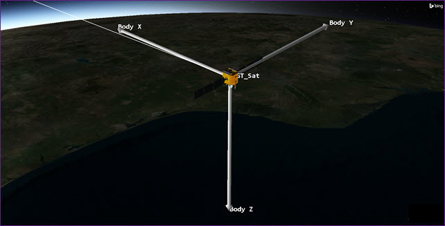
Nadir alignment with ECI velocity constraint
The Satellite (![]() ) object defaults to a Nadir alignment with ECI velocity constraint attitude. In this vehicle body frame definition, the vehicle's Z axis is aligned with the nadir direction and its X axis is constrained in the direction of the ECI velocity vector.
) object defaults to a Nadir alignment with ECI velocity constraint attitude. In this vehicle body frame definition, the vehicle's Z axis is aligned with the nadir direction and its X axis is constrained in the direction of the ECI velocity vector.
Satellite, Missile, Aircraft, Ship, and Ground Vehicle objects have one thing in common. The Body X is aligned with the direction of travel unless you change the attitude.
Selecting attitude profiles
Vehicle body frame definitions are based on attitude profiles.
- Return to RGT_Sat's () Properties ().
- Select the Basic - Attitude page.
- Change the Basic Type to ECF Velocity Alignment with Radial Constraint.
- Click .
- Bring the 3D Graphics window to the front.
ECF Velocity Alignment with Radial Constraint
The vehicle's X axis is aligned with the Earth-fixed velocity vector direction and the Z axis is constrained in the radial direction, along the position vector and opposite to geocentric nadir.
Setting the Nadir alignment back to ECI velocity constraint
- Return to RGT_Sat's () Properties () Basic - Attitude page.
- Change the Basic Type back to Nadir alignment with ECI velocity constraint
- Click .
Updating the Local Satellite Database
You must connect to the internet to update your satellite database.
There are times when you need to look at older data or you want to use local files such as your own TLE file. In this section, you'll use an archived database. You must be connected to the Internet to utilize this source.
- Open the STK_Objects_Properties's () Properties ().
- Select the Basic - Database page.
- Ensure Database Type is set to Satellite.
- Click .
Updating the Satellite Database
You can update satellite database information using Update Database Files.
| Option | Description |
|---|---|
| Update Database | Obtains the latest satellite database information from the AGI satellite database server. |
| Obtain Archived Database | Obtains an older version of the database from the date specified in the Archive Date field. If an archive is not available from the specified date, the archive for the next newest date is used instead. |
- Select the Obtain Archived Database option.
- Select Specific Database and ensure it's set to stkAllTLE (the entire database of satellites).
- Click the Database ellipsis (
 ).
). - Select the scenario folder or place the file in a folder of your choice.
- Specify the Archive Date by entering it in the text field or using the drop-down list. In this case, change the year to the previous year (e.g., if it's 2024, change it to 2022).
- Click . If an archive is not available for the specified date, the archive for the next newest data is used instead.
- When the Information window appears, click .
- Click to exit the Update Satellite Database dialog box.
- Click to accept your changes and to close the Properties Browser.
Your default save location may be in C:\ProgramData\... and this folder may be hidden. To unhide it, you must select the option in your File Explorer to show all hidden folders. Consult the help for Microsoft Windows to select that option.
Inserting a satellite from the Local Satellite Database
Use the Insert From Satellite Database tool to query a locally installed Spacecraft database.
- Insert a Satellite () object using the From TLE File () method.
- Go to the archived satellite database file (e.g., C:\Users\<username>\Documents\STK_ODTK 13\STK_Objects_Properties).
- Select stkAllTLE.tce.
- Click .
- Click when the Question window appears. Be patient, this can take a few minutes.
Using Satellite Database TLE Source
The Satellite Database TLE Source window specifies the satellite database TLE source.
- Click on the Insert From Satellite Database dialog box.
- Clear the On propagation, automatically retrieve elements check box in the Satellite Database: TLE Source dialog box. Disabling this option keeps the satellite's designated TLEs from being automatically updated next time you open the scenario.
- Click to close the Satellite Database: TLE Source dialog box.
- Click when the Question window appears. Be patient, this can take a few minutes.
- Enter 25544 in the SSC Number field.
- Click .
- Select Zarya.
- Click .
- Click to close the Insert From Satellite Database dialog box.
Viewing new versus old TLEs
Earlier you inserted ISS_ZARYA_25544 using the most current TLE. Now you've inserted the same satellite using an archived TLE that is a year old. The STK software propagated the TLE from a year ago. Any changes to the orbit during that period are not reflected. You should be able to see the difference in both the 2D and 3D Graphics windows.
- Bring the 3D Graphics window to the front.
- Click Home View () on the 3D Graphics window toolbar.
- Rearrange your view so that you can see both satellites.
- When finished, clear the ZARYA_25544 check box in the Object Browser. This turns the object off visually in both the 2D and 3D Graphics windows, but the object is still available analytically if needed.
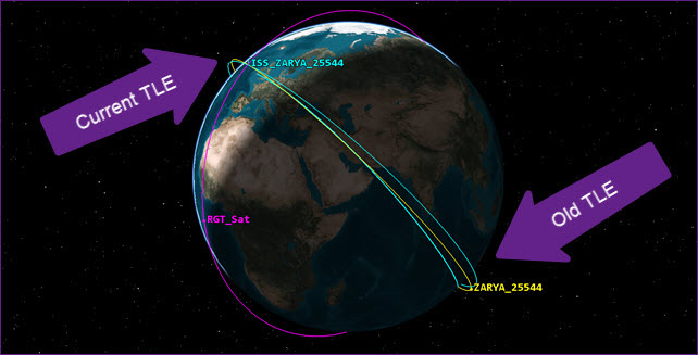
New Versus Old TLE Data
You should see a difference between using old data and new data. This is a great example why you need to use current data or data that matches your analysis period.
Inserting an Aircraft object
The Aircraft (![]() ) object models the properties and behavior of a vehicle that travels in a great arc route, generally above the surface of the earth.
) object models the properties and behavior of a vehicle that travels in a great arc route, generally above the surface of the earth.
- Bring the STK Insert Objects tool to the front.
- Insert an Aircraft () object using the Insert Default () method.
Renaming objects
It's usual to rename objects in the STK application. If you choose not to rename your objects, the STK software will name them, giving each object a number. ![]() ) object that you insert will be named Aircraft1. The next Aircraft (
) object that you insert will be named Aircraft1. The next Aircraft (![]() ) object you insert will be named Aircraft2 and so on.
) object you insert will be named Aircraft2 and so on.
- Right-click on Aircraft1 () in the Object Browser.
- Select Rename in the shortcut menu.
- Rename Aircraft1 () to My_Plane.
Changing the Aircraft object's properties
- Open My_Plane's () Properties ().
- Select the Basic - Route page.
Great Arc Propagator
At the top of the page, notice that the propagator is set to GreatArc. The Great Arc Propagator defines the route of a vehicle that follows a point-by-point path along, over, or below the surface of the Earth at a given altitude or depth. A great arc path, which lies in a plane that intersects the center of the Earth, connects the waypoints. The following Great Arc Propagator settings work with Aircraft (![]() ) , Ground Vehicle (
) , Ground Vehicle (![]() ), and Ship (
), and Ship (![]() ) objects.
) objects.
Start Time
The Start Time defaults to the scenario start time, and you can reset it. The Stop Time field is read-only and is defined by the last waypoint for the vehicle.
- Click the down arrow or right-click on the start or stop times to interact with the object time options.
- Hover over Start Time.
The shortcut gives you an idea of other selections, such as: Set to Today or Set to Tomorrow. When you enter waypoints for the object, this window enables the Replace With Time option. If you change the Start Time after you enter waypoints, all time entries in the waypoint table are updated automatically.
Route Calculation Method
You can use the Route Calculation Method shortcut menu to select the manner in which the route is calculated between each waypoint. For this tutorial, use the default Smooth Rate method.
| Option | Description |
|---|---|
| Specify Rate/Acc | Uses the Speed and Acceleration properties of each waypoint. |
| Specify Time | Uses the Time properties of each waypoint. This is useful if you want an object to stay in one spot for a period of time without moving. |
| Smooth Rate | Uses the Speed property of each waypoint. |
Selecting an altitude reference
Ground vehicles, aircraft, and ships can reference their altitude from mean sea level, terrain data, or WGS84. The World Geodetic System 1984 (WGS 84) is a three-dimensional coordinate reference frame for establishing latitude, longitude, and heights for navigation, positioning, and targeting for the DoD, IC, NATO, International Hydrographic Office, and the International Civil Aviation Organization.
Since you're currently using Terrain Server, a good rule of thumb when creating an aircraft flight route using the Great Arc Propagator is to set the altitude reference to Mean Sea Level. In the United States, mean sea level is defined as the mean height of the surface of the sea for all stages of the tide over a 19-year period.
- Open the Reference shortcut menu in the Altitude Reference panel.
- Select MSL.
Waypoints
The waypoints that comprise the great arc route are contained in a table that displays each point, along with all of its properties, in sequence. You can use the table to directly edit those properties. One row of values describes a single waypoint in the route of the vehicle.
There are two ways to enter waypoints:
- Clicking Insert Point and manually entering values.
- Clicking on the 2D Graphics window when the Basic - Route page is open.
Check out more information about the Great Arc Waypoint Properties by looking at the table with the same name on the Great Arc Waypoint Properties help page. It describes all the major position, movement, and time properties along with the calculation method.
Clicking on a map
- Leave My_Plane's () Properties () open.
- Bring the 2D Graphics window to the front by clicking on the 2D Graphic tab below the Properties Browser.
- Click somewhere in the Atlantic Ocean near the African coast and then click somewhere in the Indian Ocean near the Indian coast.
- Bring My_Plane's () Properties () back to the front.
Make sure you only click where you want a waypoint!
Notice that the Altitude, Speed, and Turn Radius values are copied for each waypoint.
Modifying a waypoint location
- Select the first waypoint.
- Select the Clicking on map changes current point check box.
- Bring the 2D Graphics window back to the front.
- Click somewhere in the Pacific Ocean near the United States coast.
- Bring My_Plane's () Properties () back to the front.
- Click until all waypoints are deleted.
- Clear the Clicking on map changes current point check box.
- Click .
Wherever you click, the STK software will move the waypoint to that location. Also, the Great Arc Propagator will automatically reroute the aircraft using the shortest distance between the waypoints. If you want to fly in a specific direction, you need to add more waypoints.
Inserting a point
You can insert waypoints manually. This is more precise than clicking on the map.
- Click .
- Enter the following by clicking in the associated cell. Press the Enter key on the keyboard after each entry:
- Click .
- Enter the following for the second waypoint:
- Click .
- Enter the following for the third waypoint:
- Click .
| Option | Value |
|---|---|
| Latitude | 38.00 deg |
| Longitude | -120.00 deg |
| Option | Value |
|---|---|
| Latitude | 30.00 deg |
| Longitude | -99.00 deg |
| Option | Value |
|---|---|
| Latitude | 40.00 deg |
| Longitude | -77.00 deg |
Viewing the waypoints in the 2D and 3D Graphics windows
My_Plane's (![]() ) flight route is located in the Continental United States.
) flight route is located in the Continental United States.
- Bring the 2D Graphics window to the front to view the flight route.
- Bring the 3D Graphics window to the front to view the flight route.
- Return to My_Plane's () Properties ().
Changing a waypoint's altitude
When modifying one waypoint, you need to know proper units. For instance, look at the first waypoint:
- The Altitude unit uses km (kilometers).
- The Speed unit uses km/sec (kilometers per second).
- The Turn Radius unit uses km.
Change the first waypoint's altitude to 20000 ft (feet).
- Select the first waypoint.
- Click inside the Altitude cell.
- Enter 20000 ft.
- Press Enter on the keyboard.
Notice the unit reverts back to the default km. My_Plane (![]() ) is flying at an altitude of 6.09600000 km (20000 ft) at the first waypoint. It slowly ascends until it reaches the second waypoint.
) is flying at an altitude of 6.09600000 km (20000 ft) at the first waypoint. It slowly ascends until it reaches the second waypoint.
Changing a waypoint's speed
Change the first waypoint's speed to 450 mi/hr (miles per hour).
- Click inside the Speed cell.
- Enter 450 mi/hr.
- Press Enter on the keyboard.
My_Plane slowly decelerates between the first and second waypoints. You can see this in the Accel cell.
Changing a waypoint's turn radius
Modify the first waypoint's turn radius to two (2) km.
- Click inside the Turn Radius cell.
- Enter 2 km.
- Press Enter on the keyboard.
- Click .
The great arc path will never reach the given waypoint unless the change in heading The direction that the aircraft is pointing. is negligible. Instead, the turn will be inscribed between the lines connecting the previous procedure to the given waypoint and the waypoint to the next procedure. The position will arrive along the line from the previous procedure toward the given waypoint and leave along the line from the given waypoint toward the next procedure. The radius of the inscribed turn will be contained to the vehicle's radius. See the figure below for a visual representation of this.
Keep this in mind when creating a movie. If your aircraft isn't flying over the location you clicked on the map or entered as a latitude and longitude, you should either decrease the turn radius or modify the waypoint location.
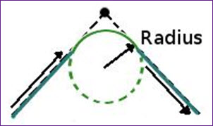
Turn Radius
Using the Set All Grid Values tool
With the Set All Grid Values tool, you can modify the Altitude, Speed, Acceleration, and Turn Radius properties for all waypoints that are currently defined in the table. The properties that can be modified using this tool will be constrained with respect to the currently selected Route Calculation Method.
- Click .
- Select Altitude, Speed, and Turn Radius in the Set All Grid Values dialog box.
- Extend the shortcut menu for Speed.
- Select nm (nautical mile).
- In the second shortcut menu, select hr (hour).
- Set the value to 500. The aircraft flies from the first to the last waypoints at a speed of 500 nautical miles per hour.
- Set the following for Altitude and Turn Radius:
- Click to close the Set All Grid Values dialog box.
- Click .
To the right of each value is a shortcut menu. These appear throughout the STK application's User Interface (UI). By clicking on them here, you can set units for Altitude, Speed, Acceleration, or Turn Radius. This comes in handy when you can't find or don't know the acronym for the unit you are looking for.
| Option | Value |
|---|---|
| Altitude | 45000 ft |
| Turn Radius | 3 km |
Setting the animation time
You can jump to a waypoint in the 2D and 3D Graphics windows.
- Select the second waypoint.
- Click inside the Time cell.
- Copy (Ctrl + C) the Time of the second waypoint.
- Right-click in the Current Scenario Time field in the Animation Toolbar.
- Select Paste.
- Click the Enter key on your keyboard.
Viewing in 3D
- Bring the 3D Graphics window to the front.
- Right-click on My_Plane () in the Object Browser.
- Select Zoom To.
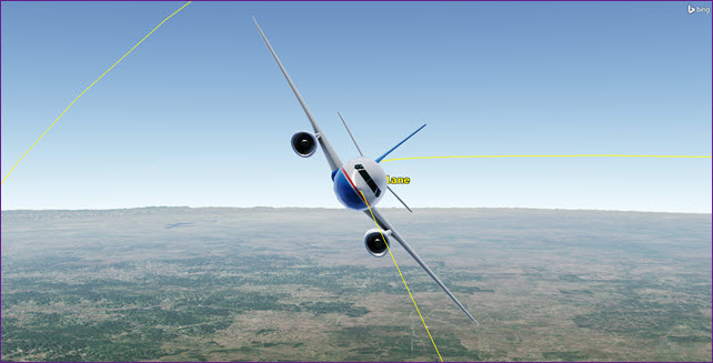
- Using the left mouse button, create a head-on view of My_Plane ().
All three waypoints are using the same values. The units converted back to the default units. The aircraft is flying the entire route at an altitude of 45000 feet MSL, at a speed of 500 nautical miles per hour and will require a turn radius of 3 kilometers at waypoint two. My_Plane (![]() ) is in the middle of the turn. Notice that there is no roll (banking) associated with the attitude.
) is in the middle of the turn. Notice that there is no roll (banking) associated with the attitude.
No Roll in Turn
Attitude Profiles
The STK application is set by default to the Standard attitude option, which enables you define a vehicle's attitude profile
You can apply attitude changes to all moving objects in STK: Aircraft, Ground Vehicles, Missiles, Satellites, and Ships.
- Leave the view in the 3D Graphics window.
- Return to My_Plane's () Properties ().
- Select the Basic - Attitude page.
Choosing the Coordinated Turn attitude
This profile computes the roll (banking) of an aircraft based on a balancing of the forces acting on the aircraft, assuming a zero angle of attack The angle between the body X axis and the projection of the velocity vector onto the body XZ plane. The velocity vector is the velocity of the object as observed in the object's central body fixed coordinate system. and no slip condition. ![]() ) object which is acting as a camera's field of view. Maybe you're making a movie and you want the Aircraft (
) object which is acting as a camera's field of view. Maybe you're making a movie and you want the Aircraft (![]() ) object to roll like a real aircraft.
) object to roll like a real aircraft.
- Open the Type drop-down list in the Basic panel.
- Select Coordinated Turn.
- Leave the Time Offset at 10 sec.
- Click .
Viewing in 3D
- Bring the 3D Graphics window back to the front.
- Click Reset () in the Animation Toolbar.
Coordinated Turn
The aircraft is now banking (roll). The severity of the roll is determined by the speed and turn radius of the plane.
Setting 2D Graphics properties
2D Graphics Attributes answer three basic questions about an STK object:
- What do you want to show?
- How do you want it to look?
- When do you want it to be seen?
You can make changes to the way the STK software displays your aircraft's path.
- Return to My_Plane's () Properties ().
- Select the 2D Graphics - Attributes page.
- Change Color, Line Style, and Line Width to whatever selections you want.
- Click .
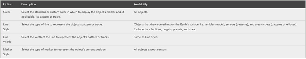
2D Graphics Attributes Properties
Viewing in the Graphics windows
- Bring the 2D Graphics window to the front.
- Zoom in or out to get a good view of MyPlane's () flight route.
- When finished, bring the 3D Graphics window to the front.
- If needed, zoom to My_Plane ().
Changes made in the 2D Graphics Properties are applied to both the 2D Graphics and 3D Graphics windows.
Setting 3D Graphics properties
Unlike 2D Graphics properties, which apply to both the 2D and 3D Graphics windows, 3D Graphics properties only apply to the 3D Graphics window.
Use the 3D Graphics Properties - Vector to do the following:
- Control the display of vectors and other geometric elements, such as axes and angles, related to the Earth or other central body in the selected 3D Graphics window.
- Control the display of vectors and other geometric elements related to the selected object.
Follow these steps:
- Return to My_Plane's () Properties ().
- Select the 3D Graphics - Vector page.
- Ensure the Vectors tab is selected.
- Select the Show check box for Sun Vector.
- Select the Axes tab.
- Select the Show check box for Body Axes.
- Click .
Viewing in 3D
- Bring the 3D Graphics window to the front.
- If needed, Zoom To My_Plane ().
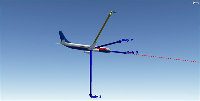
Body Axes and Sun Vector
Animating the scenario
The body axes remain fixed throughout the flight. Even when the Sun drops below the horizon, the sun vector continuously stays locked on the Sun.
- Decrease Time Step (
 ) to five (5.00) seconds in the Animation Toolbar.
 - Click Start () to animate the scenario.
- Click Reset () when finished.
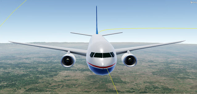
Using a 3D Graphics model
You can specify a model to represent a given vehicle, facility, place, or target in the 3D Graphics window.
Supported model file types are:
Support for 3D models using the COLLADA (.dae) format has been deprecated. To maximize future compatibility, COLLADA models used in STK scenarios should be converted to the gLTF model format, using any of the readily available 3D modeling content creation tools such as Blender, Maya, or Modo.
Select a model for your aircraft.
- Return to My_Plane's () Properties ().
- Select the 3D Graphics - Model page. The current model you see in the 3D Graphics window is the aircraft.glb.
- Click the Model File ellipsis () in the Model panel. All the models shown in the File dialog box come with the STK software install.
- Select any model you'd like to use in the scenario.
- Click to change to your selected model.
- Click to apply your changes and close the Properties Browser.
- Bring the 3D Graphics window to the front. You have a new model type representing the Aircraft () object.
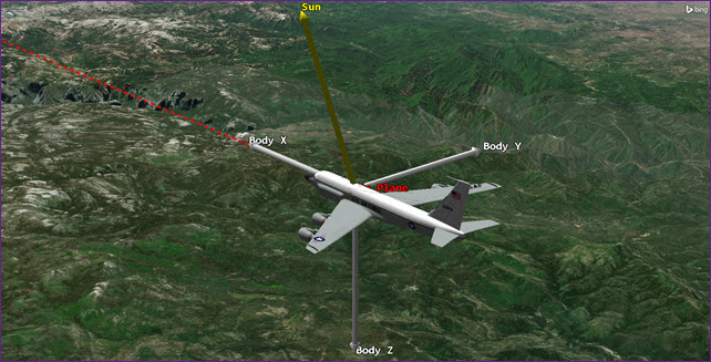
RC-135 Rivet Joint Model
Area Target object
The Area Target object (![]() ) models a region on the surface of the central body.
) models a region on the surface of the central body.
Selecting the Countries And US States method
This insert method, available on the Insert STK Objects tool, enables you to add one or more US states or countries as area targets. By default, the list displays both countries and US states.
- Insert an Area Target () object using the Countries and US States (
 ) method.
 - Select United_States_of_America when the Select Countries And US States dialog box opens. Notice that the Insert field becomes active.
- Keep the default selection of Primary Area Only.
- Click .
- Click .
Area targets are created from shapefiles, which contain one or more polygons. Each polygon is converted into one area target. If the shapefile for the selected area contains two or more polygons, you can choose whether to add only the largest polygon (Primary Area Only) or all polygons (All Areas) in the shapefile.
Viewing in 2D
- Bring the 2D Graphics window to the front.
- Zoom out far enough so you can see the Area Target, Hawaii, and Alaska.
This is a good example of Primary Area Only and All Areas. Had you selected All Areas, you'd see all of Alaska and all the Hawaiian Islands enclosed in area targets.
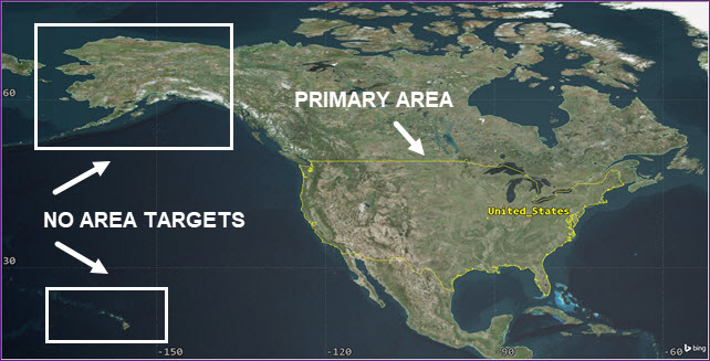
United States Area Target Primary Area Only
Using the Area Target Wizard method
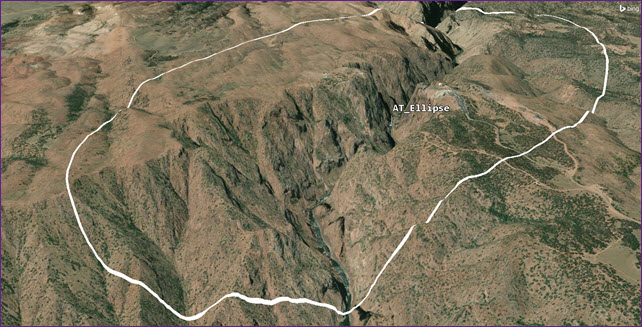
Use the Area Target Wizard to add an area target, define its perimeter, and set its graphic properties. There are two types of Area Targets: ellipse and pattern. Using the Area Target Wizard, create an ellipse.
- Insert an Area Target () object using the Area Target Wizard (
 ) method.
 - Set the following in the Area Target Wizard:
- Click .
| Option | Value |
|---|---|
| Name | AT_Ellipse |
| Area Type | Ellipse |
| Semi-Major Axis | 2 km |
| Semi-Minor Axis | 1 km |
| Bearing | 132.353 deg |
| Centroid | Latitude 38.4613 deg / Longitude -105.3256 deg |
Viewing in 3D
- Bring the 3D Graphics window to the front.
- Right-click on AT_Ellipse () in the Object Browser.
- Select Zoom To.
- Use your mouse to zoom out until you can see the entire area target.
- Using your left mouse button, move your view around in circles. Note how the label gets "lost" in the terrain.
Changing 3D Graphics window properties - Label Declutter
Label Declutter raises labels from the central body and toward the viewer, keeping the labels from being obscured by the terrain. This is especially helpful if you label is at the bottom of a valley or canyon.
- Click Properties () on the 3D Graphics window toolbar.
- Select the Details page.
- Select the Enable check box in the Label Declutter panel.
- Click .
Notice how the label appears above the surface of the terrain.
Area Target Ellipse Using Label Declutter
Using the Insert Default method
Insert Default adds the selected object and applies the default settings to the newly added object.
- Insert an Area Target () object using the Insert Default () method.
- Rename AreaTarget3 () to Local_Airfield.
Defining the Area Target
Specify the location of the Area Target.
- Open Local_Airfield's () Properties ().
- Select the Basic - Boundary page.
- Click four (4) times.
- Set the following Latitude and Longitude values for the Points in the order shown (simply copy and paste from the tutorial):
- Click .
The Basic - Boundary page is similar to the Area Target Wizard except you don't get a small 2D Graphic view. Now you'll outline a local airfield. Maybe you're trying to determine when a Satellite (![]() ) object or an Aircraft (
) object or an Aircraft (![]() ) object sees the airfield.
) object sees the airfield.
| Latitude | Longitude |
|---|---|
| 38.4345 deg | -105.116 deg |
| 38.4267 deg | -105.0999 deg |
| 38.4256 deg | -105.1008 deg |
| 38.4333 deg | -105.117 deg |
Viewing in 3D
- Bring the 3D Graphics window to the front.
- Zoom To Local_Airfield ().
- Use your mouse to get a good view of the area target outlining the airfield.
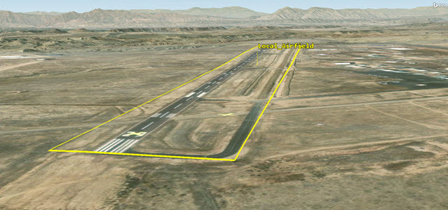
Area Target Local Airfield
Inserting a Facility object
The Facility object (![]() ) models a ground station or other facility on the surface of the central body. Similar to Place (
) models a ground station or other facility on the surface of the central body. Similar to Place (![]() ) and Target (
) and Target (![]() ) objects property wise, what makes a Facility (
) objects property wise, what makes a Facility (![]() ) object stand out is when you insert one using the standard object database.
) object stand out is when you insert one using the standard object database.
- Insert a Facility () object using the From Standard Object Database () method.
- Enter Castle Rock in the Name field on the Search Standard Object Data dialog box.
- Click .
- Take a look at the Results.
- Change Name to White Sands.
- Click .
- Delete White Sands from the Name field.
Notice that the first result gives you information such as role, country, and status. If you insert the first selection it is downloaded from the online source: AGI's Standard Object Data Service. The other two results were part of the STK software install and come from the install area on your hard drive.
White sands has many more selections to include ground stations, launch pads, and launch sites.
Inserting Intelsat
- Scroll down to the Network field.
- Open the Network drop-down list.
- Select INTELSAT.
- Click .
This enables you to quickly add all the Facility (![]() ) objects associated with that network.
) objects associated with that network.
Entering White Sands - SULF
- Change Network back to no selection (-).
- Enter White Sands in the Name field.
- Click .
- In the Results list, select White Sands - SULF.
- Click .
- Click to close the Search Standard Object Data dialog box.
Editing SULF's properties
- Open White - Sands SULF's () Properties ().
- Select the Basic - Position page.
- Select the Use terrain data check box.
- Click .
The Use terrain data option overrides the altitude used by the Facility (![]() ) object, which now uses Terrain Server's terrain as an altitude reference. This is unique to the Facility (
) object, which now uses Terrain Server's terrain as an altitude reference. This is unique to the Facility (![]() ) object. The default altitude was most likely based on a terrain file other than the terrain used by Terrain Server. If Terrain Server is disabled, then the Facility (
) object. The default altitude was most likely based on a terrain file other than the terrain used by Terrain Server. If Terrain Server is disabled, then the Facility (![]() ) object references the surface of the WGS84 Ellipsoid.
) object references the surface of the WGS84 Ellipsoid.
Viewing in 3D
- Bring the 3D Graphics window to the front.
- Zoom to White - Sands SULF ().
The Facility (![]() ) object is located at the launch pad at White Sands.
) object is located at the launch pad at White Sands.
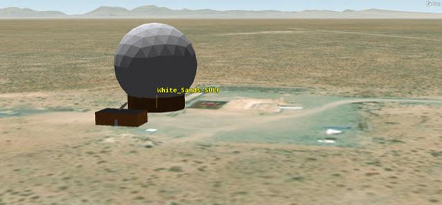
White Sands SULF
Removing the azimuth-elevation mask
Looking at White - Sands SULF (![]() ), you can see a visual representation of an azimuth-elevation mask. You can use an azimuth-elevation mask to constrain access to the object. The mask can come from terrain or a custom az-el mask. Turn off the mask file.
), you can see a visual representation of an azimuth-elevation mask. You can use an azimuth-elevation mask to constrain access to the object. The mask can come from terrain or a custom az-el mask. Turn off the mask file.
- Select the Basic - AzElMask page.
- Open the Use drop-down list.
- Select None.
- Clear the Use Mask for Access Constraint check box.
- Click .
Inserting a Ground Vehicle object
The Ground Vehicle (![]() ) object models the properties and behavior of a vehicle that travels in a great arc route on the surface of the earth. The great arc propagator works exactly the same for a ground vehicle as it does for an Aircraft (
) object models the properties and behavior of a vehicle that travels in a great arc route on the surface of the earth. The great arc propagator works exactly the same for a ground vehicle as it does for an Aircraft (![]() ) object.
) object.
- Insert a Ground Vehicle () object using the Insert Default () method.
- Rename GroundVehicle1 () to ATV.
- Open ATV's () Properties ().
Setting the reference terrain
Unlike the Aircraft (![]() ) object, the Ground Vehicle (
) object, the Ground Vehicle (![]() ) object is on the surface of the terrain. You need to take that into account.
) object is on the surface of the terrain. You need to take that into account.
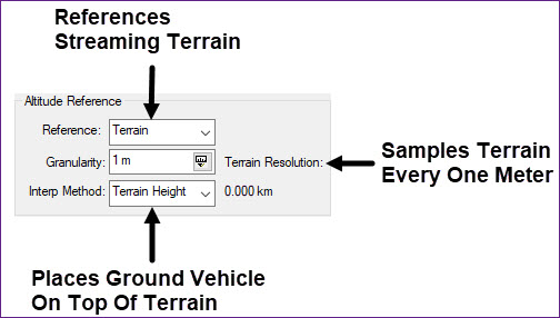
Great Arc Referencing Terrain
- Select the Basic - Route page.
- Set the following in the Altitude Reference panel:
| Option | Value |
|---|---|
| Reference | Terrain |
| Granularity | 1 m |
| Interp Method | Terrain Height |
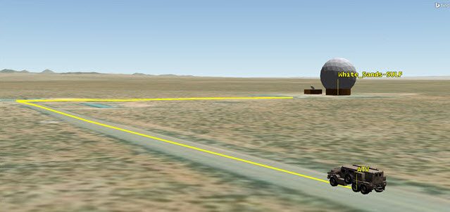
Creating waypoints
ATV (![]() ) is driving down the road to the launch pad at White_Sands-SULF (
) is driving down the road to the launch pad at White_Sands-SULF (![]() ).
).
- Click .
- Set the waypoint parameters as specified below; you can copy and paste to save time:
- Click .
- Specify the parameters for the second waypoint:
- Click .
- Specify the parameters for the third waypoint:
| Option | Value |
|---|---|
| Latitude | 33.71868 deg |
| Longitude | -106.73949 deg |
| Option | Value |
|---|---|
| Latitude | 33.72085 deg |
| Longitude | -106.73928 deg |
| Option | Value |
|---|---|
| Latitude | 33.72085 deg |
| Longitude | -106.73731 deg |
Setting the speed and altitude
Keep in mind that the center point of the ground vehicle is right on top of the terrain. You might want to raise it a foot or so depending on your analysis. The object center point, unless changed, is where analysis for the object takes place. Also, terrain undulation could be a factor. The ground vehicle could appear, visually, to dart into and out of terrain, especially when modeling in an area containing rugged terrain. Terrain resolution can be a factor too.
All ground object center points start on the WGS84 or terrain surface.
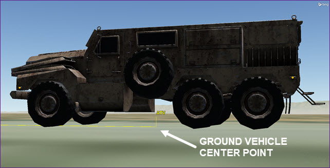
Ground Vehicle Center Point
- Click
- Select the Altitude and Speed check boxes in the Set All Grid Values dialog box.
- Specify the parameters for the waypoints:
- Click to close the Set All Grid Values dialog box.
- Click to apply all changes and close the properties browser.
| Option | Value |
|---|---|
| Altitude | 1 ft |
| Speed | 15 mi/hr |
Viewing in 3D
- Bring the 3D Graphics window to the front.
- Zoom To ATV ().
- Select X Real-time Animation Mode (
 ) in the Animation Toolbar.
 - Click Start () to animate the scenario.
- Click Reset () when finished.
ATV Driving At White Sands
Inserting a Target object
The Target object (![]() ) models a point of interest on the surface of the central body. The properties are identical to the Place (
) models a point of interest on the surface of the central body. The properties are identical to the Place (![]() ) and Facility (
) and Facility (![]() ) objects.
) objects.
- Insert a Target () object using the Define Properties () method.
- Select the Basic - Position page.
- Set the following:
- Click .
- Rename Target1 () to Missile_Tgt.
| Option | Value |
|---|---|
| Latitude | 32.9 deg |
| Longitude | -106.3 deg |
Viewing in 3D
- Bring the 3D Graphics window to the front.
- Zoom To Missile_Tgt ().
- Zoom out so you can see both White_Sands-SULF () and Missile_Tgt ().
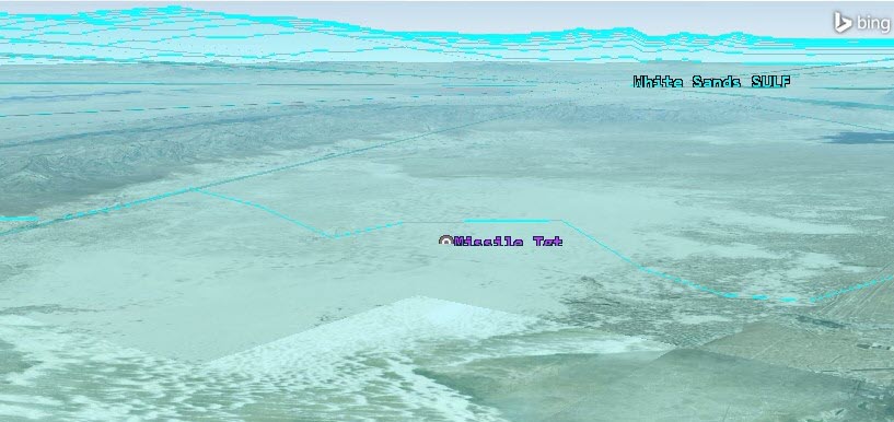
Missile Tgt in the White Sands SULF Area Target
You are going to launch a sounding rocket from White_Sands-SULF (![]() ) so that it impacts Missile_Tgt (
) so that it impacts Missile_Tgt (![]() ).
).
Inserting a Missile object
The Missile (![]() ) object models the properties and behavior of a vehicle following an elliptical path that begins and ends at the surface of the central body.
) object models the properties and behavior of a vehicle following an elliptical path that begins and ends at the surface of the central body.
- Insert a Missile () object using the Insert Default () method.
- Rename Missile1 () to Sounding_Rocket.
- Open Sounding_Rocket's () Properties ().
- Select the Basic - Trajectory page.
- Notice the Propagator is Ballistic.
Using the Ballistic Propagator
The Ballistic Propagator defines an elliptical path that begins and ends at the Earth's surface. Specifying a fixed flight time, initial velocity or altitude can further refine the shape of the trajectory.![]() ) and impacting Missile_Tgt (
) and impacting Missile_Tgt (![]() ).
).
- Clear the check box next to White_Sands_SULF () in the Object Browser.
- Return to Sounding_Rocket's () Properties () Basic - Trajectory page.
- Set the following:
- Click .
The Facility (![]() ) object is still there, and you can use it analytically. Disabling the option disables it visually.
) object is still there, and you can use it analytically. Disabling the option disables it visually.
| Option | Value |
|---|---|
| Launch Latitude - Geodetic | 33.7212 deg |
| Launch Longitude | -106.7364 deg |
| Launch Altitude | 4750 ft (compensate for terrain) |
| Change Fixed Delta-V to Fixed Apogee Alt | 100 km |
| Impact Latitude - Geodetic | 32.9 deg |
| Impact Longitude | -106.3 deg |
| Impact Altitude | 3910 ft (compensate for terrain) |
Viewing in 3D
- Bring the 3D Graphics window to the front.
- Zoom To Sounding_Rocket ().
- Click Increase (
 ) Time Step in the Animation Toolbar to set the X Real Time Multiplier to 8.00.
 - Click Start () to animate the scenario.
- Click Reset () when finished.
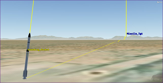
Sounding Rocket and Target
Inserting a Place object
The Place (![]() ) object models a point of interest on the surface of the central body.
) object models a point of interest on the surface of the central body.
Using the Search by Address method
- Insert a Place () object using the Search by Address () method.
- Enter Pikes Peak in the Enter an address or other search criteria below field when the STK: Insert by Address dialog box opens.
- Select Pikes Peak, CO, in the Results list.
- Click .
- Click to close the STK: Insert by Address dialog box.
- Zoom To Pikes_Peak_CO().
- Bring the 3D Graphics window to the front.
The Insert by Address option requires an internet connection. If you do not have an internet connection, you can select the Define Properties option and set the lat/lon manually to 38.8409, - 105.0423.
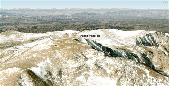
Search by Address / Pikes Peak Colorado
Using the Insert Default method
- Insert a Place () object using the Insert Default () method.
- Zoom To Place1 ().
- Bring the 3D Graphics to the front.
The Place (![]() ) object may have a different number than the one in this tutorial. If you have entered other Place (
) object may have a different number than the one in this tutorial. If you have entered other Place (![]() ) objects prior to this, it may be something like Place2, Place3, etc.
) objects prior to this, it may be something like Place2, Place3, etc.
A Place (![]() ) object or a Facility (
) object or a Facility (![]() ) object will default to AGI Headquarters.
) object will default to AGI Headquarters.
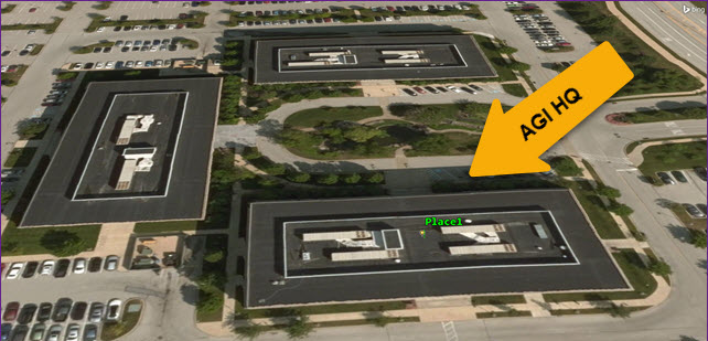
Place Object Insert Default / AGI Headquarters
Using the From City Database method
- Insert a Place () object using the From City Database () method.
- Enter Exton in the Name field when the Search Standard Object Data dialog box opens.
- Click .
- Right-click on Exton/Pennsylvania in the Results list.
- Select Insert Selected Item. This is another way to insert an item from the database.
- Click to close the Search Standard Object Data dialog box.
Viewing in 3D
- Bring the 3D Graphics window to the front.
- Using your right mouse button or the mouse scroll wheel, zoom out from Place1 () until you see Place1 ())
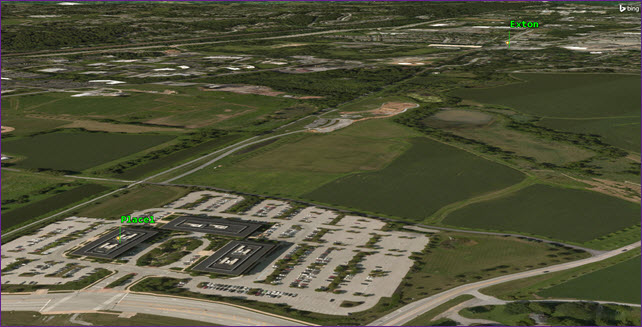
Exton and Place1
The From City Database method inserts the city using a centroid for the city area. If you need an exact location, use the Search by Address method or the following procedure.
Moving Place1 by clicking the 2D Graphics window
When you have a Facility (![]() ), Place (
), Place (![]() ) or Target (
) or Target (![]() ) object's properties open and you are on the Basic - Position page, you can move the object to a desired location by clicking on the 2D Graphics window. Move Place 1 (
) object's properties open and you are on the Basic - Position page, you can move the object to a desired location by clicking on the 2D Graphics window. Move Place 1 (![]() ) to the top-left corner of the building where a sensor is located.
) to the top-left corner of the building where a sensor is located.
- Bring the 2D Graphics window to the front.
- Zoom to Place1 (). Remember, in the 2D Graphics window, you have to use your mouse to center and zoom to an object!
- Open Place1's () Properties ().
- Return to the 2D Graphics window.
- Click the upper-left corner of the building.
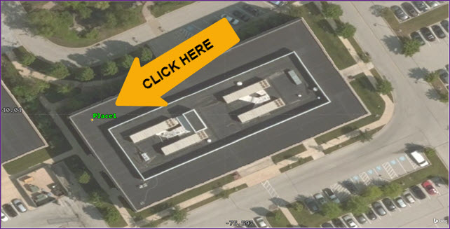
Move Place1 on 2D Graphics Window
Setting the height above ground of the facility
Set Place1 (![]() ) 30 feet above the ground to model the sensor on the roof of the building.
) 30 feet above the ground to model the sensor on the roof of the building.
- Return to Place1's () Properties ().
- Enter 30 ft in the Height Above Ground field.
- Click .
All these steps were purposeful. You moved Place1 (![]() ) to the upper-left corner of the building because there is a sensor located at that spot. Furthermore, the building's roof is 30 feet above the ground. These steps were used to put the Place1 (
) to the upper-left corner of the building because there is a sensor located at that spot. Furthermore, the building's roof is 30 feet above the ground. These steps were used to put the Place1 (![]() ) in the correct location for future analysis with the STK software.
) in the correct location for future analysis with the STK software.
Using the 3D Object Editor
Use the 3D Object Editor to define and modify the position of an area target, facility, place, aircraft, ground vehicle, ship, or target in the 3D Graphics window.
- Bring the 3D Graphics window to the front.
- Click Orient from Top (
 ) in the 3D Graphics window toolbar.
 - Zoom To Place1 ().
- Open the 3D Editing Object drop-down list.
- Select Place/Place1.
- Click Object Edit Start/Accept (
 ) to start the editing process.
 - Press the Shift key on your keyboard.
- Left-click in the center of the building.
- Click Object Edit Cancel (
 ) because that is not where you want to object to go.
This is an easy way to add or move a place object. However, that's not where you want this object to go this time.
Fixing the location
- Click Object Edit Start/Accept () to start the editing process.
- Press the Shift key on your keyboard.
- Left-click in the upper-right corner of the building.
- Click Object Edit Start/Accept (
 ) to accept the change.
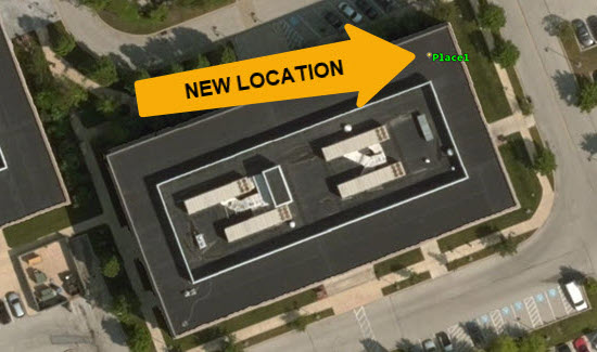
Move Place1 with the 3D Object Editor
Inserting a Ship object
The Ship (![]() ) object models the properties and behavior of a ship. Like the Aircraft (
) object models the properties and behavior of a ship. Like the Aircraft (![]() ) object and the Ground Vehicle (
) object and the Ground Vehicle (![]() ) object, the Ship (
) object, the Ship (![]() ) object uses the Great Arc propagator. You can use the 3D Object Editor to create waypoints for the Ship (
) object uses the Great Arc propagator. You can use the 3D Object Editor to create waypoints for the Ship (![]() ) object.
) object.
- Insert a Ship () object using the Insert Default () method.
- Rename Ship1 () to MyShip.
Viewing in 3D
- Bring the 3D Graphics window to the front.
- In the 3D Graphics window toolbar, click Home View ().
- In the 3D Graphics window toolbar, use Zoom In (
 ) to recenter your view off the east coast of the United States.
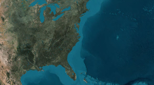
East Coast of the United States Centered
Changing the Ship object waypoints
- Open the 3D Editing Object drop-down list.
- Select Ship/MyShip.
- Click Object Edit Start/Accept () to start the editing process.
- Press the Shift key on your keyboard.
- Left-click somewhere in the Atlantic Ocean off the northeast coast of the United States.
- Press the Shift key on your keyboard.
- Left-click somewhere in the Atlantic Ocean off the southeast coast of the United States. MyShip () will move north to south.
- Click Object Edit Start/Accept () to accept the change.
Setting the MyShip altitude reference
Since you're using streaming terrain (Terrain Server), its a good idea to reference Mean Sea Level for the ship.
- Open MyShip's () Properties ().
- Select the Basic - Route page when the Properties Browser opens.
- Open the Reference drop-down list in the Altitude Reference panel.
- Select MSL.
- Click .
You can make any other changes, such as speed, as required.
Modifying a Waypoint
You want to modify a waypoint. You can use the 3D Object Editor.
- Bring the 3D Graphics window to the front.
- Zoom To MyShip ().
- Click Orient from Top () in the 3D Graphics window toolbar.
- Ensure Ship/MyShip is still showing in the 3D Object Editing drop-down list.
- Click Object Edit Start/Accept () to start the editing process.
- Place your cursor on MyShip's () waypoint.
- Hold down your left mouse button to drag MyShip's () waypoint to a different location.
- Click Object Edit Start/Accept () to accept the change.
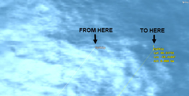
MyShip Waypoint
Viewing in 3D
Just like you did with the Ground Vehicle (![]() ) object and the Aircraft (
) object and the Aircraft (![]() ) object, you can watch your scenario animate in real time:
) object, you can watch your scenario animate in real time:
- Click Start () in the Animation Toolbar to animate your scenario.
- Click Reset () when finished.
Adding a Sensor object
The Sensor (![]() ) object models the field of view and other properties of a sensing device attached to another STK object.
) object models the field of view and other properties of a sensing device attached to another STK object.
- Insert a Sensor (
 ) object using the Insert Default () method.
 - Select White_Sands-SULF () in the Select Object dialog box.
- Click .
- Rename Sensor1 () to WS_Sensor.
Viewing in 3D
- Bring the 3D Graphics window to the front.
- Zoom To White_Sands-SULF ().
- Select the check box next to White_Sands-SULF () in the Object Browser. This will turn it back on visually.
Adding White Sands situational awareness
If you're going to use the Sensor (![]() ) object analytically, to include a report containing an azimuth, remember the following: A report such as an Azimuth, Elevation, Range (AER) report is calculated with respect to the parent object. You can learn more about AER reports in Lesson Three: Access Reports and Graphs.
) object analytically, to include a report containing an azimuth, remember the following: A report such as an Azimuth, Elevation, Range (AER) report is calculated with respect to the parent object. You can learn more about AER reports in Lesson Three: Access Reports and Graphs.
- Open White_Sands-SULF's () Properties ().
- Select the 3D Graphics - Vector page.
- Select the Axes tab.
- Click
- Select White_Sands-SULF () in the Object List on the left.
- Select Body (
 ) in the Installed Components folder in the Components for: White_Sands-SULF list on the right.
 - Click .
- Click to accept your changes and to close White_Sands-SULF's () Properties ().
This opens the Vector Geometry Tool (VGT), which is part of the the STK software's Analysis Workbench capability. VGT contains components that define location, pointing, and orientation in 3D space.
Viewing in 3D
- Return to the 3D Graphics window.
- Use your mouse to zoom in on White_Sands-SULF () to view the body axes.
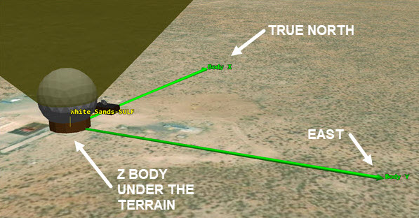
Facility Object Body Axes
Adjusting the Sensor orientation
The Sensor (![]() ) object can see out to the stars. Using the body axes on the parent object, you can visualize where the sensor is looking. Set up WS_Sensor (
) object can see out to the stars. Using the body axes on the parent object, you can visualize where the sensor is looking. Set up WS_Sensor (![]() ) so that it covers a field of view of 180 degrees and has a limited range of 1000 kilometers (km).
) so that it covers a field of view of 180 degrees and has a limited range of 1000 kilometers (km).
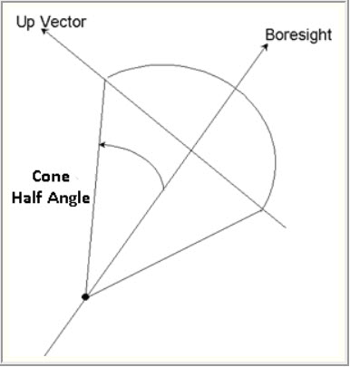
- Open WS_Sensor's () Properties ().
- Select the Basic - Definition page.
- In the Simple Conic panel, enter 90 deg in the Cone Half Angle field.
- Click .
A Simple Conic sensor pattern (default type) is defined by a simple cone angle. In this case, it defaults to a cone half-angle of 45 degrees, which means you have a 90-degree field of view.
Cone Half Angle
Checking the Sensor pointing
The Pointing page enables you to set parameters to determine how a sensor is aimed. The Fixed pointing type enables you to specify the orientation of the sensor with respect to the body frame of your parent object. While the sensor remains fixed relative to the parent object, motion of the parent object changes the direction in which the sensor is pointing.
- Select the Basic - Pointing page.
- Notice that the Pointing Type defaults to Fixed.
Understanding the Fixed Type
Facility, place, and target objects have body-fixed coordinate axes, which align the X axis along local horizontal North direction, the Y axis along local horizontal East direction, and the Z axis along local Nadir direction (i.e., opposite to local surface normal). Therefore:
The Sensor (![]() ) object defines azimuth based off the Facility (
) object defines azimuth based off the Facility (![]() ) object's X axis and elevation as an angle measured from the X-Y plane toward the negative Z axis, i.e., in a manner that makes positive elevation look up from the local horizontal plane.
) object's X axis and elevation as an angle measured from the X-Y plane toward the negative Z axis, i.e., in a manner that makes positive elevation look up from the local horizontal plane.
About Boresight - Rotate:
- The Z axis is aligned with the boresight.
- The Y axis runs along the intersection of the subcomponent reference X-Y plane and the parent body X-Y plane.
- The X-Y plane is perpendicular to the sensor or antenna boresight so that it forms an azimuth angle with the parent reference Y axis.
Setting constraints
Using the Constraints - Active page enables you to impose constraints on an object.
- Select the Constraints - Active page.
- Note the currently used constraints.
- Line of Sight: Access to the object is limited to lines of sight not obstructed by the ground, which in this instance is the central body.
- Field-of-View (Sensors only): Access is denied if the associated object is not within the field of view as defined by the angle settings for the sensor.
- Click Add new constraints (
 ) in the Active Constraints toolbar.
 - Select Range in the Constraint Name list when the Select Constraints to Add dialog box opens.
- Click .
- Click to close the Select Constraints to Add dialog box.
- Select the Max check box in the Range panel.
- Enter 1000 km in the Max field.
- Click .
Range is measured as the distance between the two objects.
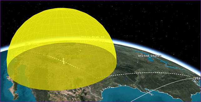
Viewing in 3D
- Bring the 3D Graphics window to the front.
- Zoom out until you can see WS_Sensor's () field of view.
Sensor Object field-of-view
WS_Sensor (![]() ) only sees other objects when they are inside of or passing through its field of view.
) only sees other objects when they are inside of or passing through its field of view.
Inserting a rectangular Sensor object
Rectangular sensor types are typically used with satellites or aircraft for modeling the field of view of instruments such as push broom sensors and star trackers.
- Insert a Sensor () object using the Insert Default () method.
- Select RGT_Sat () in the Select Object dialog box.
- Click .
- Rename the Sensor () to Sat_Sensor.
- Bring the 3D Graphics window to the front.
- Zoom to RGT_Sat ().
- Use your mouse to zoom out until you can see Sat_Sensor's () field of view.
Unlike the Sensor (![]() ) object attached to a Facility (
) object attached to a Facility (![]() ) object that points up, a Sensor (
) object that points up, a Sensor (![]() ) object attached to an airborne object (e.g., Satellite (
) object attached to an airborne object (e.g., Satellite (![]() ) object) points down.
) object) points down.
Defining the Sensor's properties
- Open Sat_Sensor's () Properties ().
- Select the Basic - Definition page.
- Set the following:
- Click .
- Bring the 3D Graphics window to the front.
- Change the view so that the sensor is visible between the satellite and the surface of the Earth.
| Option | Value |
|---|---|
| Sensor Type | Rectangular |
| Vertical Half Angle | 20 deg |
| Horizontal Half Angle | 10 deg |
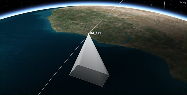
Rectangular Sensor
Redirecting the Sensor
The sensor is pointing straight down with its boresite directed along the satellite's body Z axis. By default, when you attach an object onto a satellite, the object points in the body +Z direction. Here, you will point the sensor in a different direction.
- Return to Sat_Sensor's () Properties ().
- Select the Basic - Pointing page.
- Set the following:
- Click .
- Click .
| Option | Value |
|---|---|
| Azimuth | 270 deg |
| Elevation | 60 deg |
The first thing you may notice when you click is that the Azimuth setting went from 270 deg to -90 deg. You see this throughout the STK application. The original Azimuth of 0 deg placed the sensor's boresite along the body X axis. The original Elevation setting of 90 deg swung that boresite so that it was pointing down along the body Z axis. So, if you set both the Azimuth and Elevation settings to 0 deg, the sensor's boresite would be pointing along the satellite's orbital path.
Viewing in 3D
- Bring the 3D Graphics window to the front.
- Select Normal Animation Mode () in the Animation Toolbar.
- Click Decrease Time Step () to set the Time Step to one (1) sec.
- Click Start () to animate the scenario. Any objects that pass through the sensor's field of view will be seen by the sensor.
- Click Reset () when finished.
- Save () your work.
Redirected Boresite
The boresite is now pointing along the negative body Y (Azimuth: 270 deg OR -90 deg) and the boresite is elevated 30 degrees (Elevation: 60 deg) from the satellite's body Z.
Closing the scenario
Save your work and close out of your scenario.
- Close any open windows except for the 2D and 3D Graphics windows.
- Save () your work.
- Select the File menu in the Menu Bar.
- Select Close to close your scenario without closing the STK application.
Summary
This tutorial began with understanding the purpose of the Insert STK Objects tool. Next, the Scenario (![]() ) object and its properties were discussed. This was followed by an in-depth discussion of commonly used object in the Insert STK Objects tool, how to insert objects into the scenario, and which method to use during that insertion.
) object and its properties were discussed. This was followed by an in-depth discussion of commonly used object in the Insert STK Objects tool, how to insert objects into the scenario, and which method to use during that insertion.
Continue to Lesson Three: Access Reports and Graphs.
On your own
Open the Insert STK Objects tool and select Edit Preferences. Enable the following objects:
- Launch Vehicle: The Launch Vehicle (
 ) object models the properties and behavior of a vehicle that follows an ascent trajectory from a launch point to an orbit insertion point.
 - Line Target: The Line Target (
 ) object models a linear region of interest on the surface of a central body.
 - Planet: The Planet (
 ) object models orbital and other properties of a planet, a moon, an asteroid, or the sun.
 - Star: The Star object models position, proper motion, annual parallax, visual magnitude, and other properties of a star.
Explore the capabilities of these additional objects.